
This text has been translated by a machine and has not been reviewed by a human yet. Apologies for any errors or approximations – do not hesitate to send us a message if you spot some!
Economic players, whether private or public, project themselves into the future and prepare for it by investing (e.g. in a new machine for a company, in infrastructure for a state or local authority, in a company’s capital for a financial player).
An important economic question is whether this investment will be profitable, i.e. whether it will generate at least as much income as it cost. It should be noted here that the terms profitability, income, profit or costs do not necessarily have the same meaning for all economic players: a financier or company director will tend to look primarily (or even solely) at the financial dimension; a State or local authority will adopt a broader understanding of profitability, including benefits and costs for society, or the natural environment.
In all cases, time projection poses a difficult question: how can we assess the economic effects of events occurring over a long period, and how can we add together those that will take place over the next few years and those that will occur over the longer term?
To answer this question, economists use a tool: the discount rate, which converts future values into today’s values. It’s a key parameter for factoring time into financial calculations.
The question of the discount rate is also at the heart of attempts to assess the long-term economic impacts of the climate crisis, and more generally the future ecological impacts of projects.
In this fact sheet, we explain the discounting mechanism, how it is used and chosen in the sphere of private investment, and then in that of public investment. Finally, we detail its implications for the fight against climate change, as well as the main positions taken by economists on the subject.
Understanding the discounting mechanism
Discounting is the technique of reducing values received (or spent) at different points in time to a present value. It enables us to compare monetary sums today with sums in the future.
Intuitive perception of the discounting concept
Let’s start with a simple question: given a constant income and price level, would you rather receive €100 today or €101 a year from now? You’ll probably answer €100 today, either out of impatience to get the money, or out of immediate necessity, or to enjoy it for sure, because who knows what tomorrow will bring?
Let’s rephrase this question differently. Instead of asking whether you’d prefer to receive money today or later, ask yourself how much you’d be willing to give up to receive €100 today.
Your answer will probably be between €100 and €110, perhaps higher for some.
Translated into economic terms, you have just discounted the sum you expect to receive in the future, i.e. reduced it to the value it represents for you today.
The discount rate is in a way the inverse of the interest rate.
If you invest €100 in an interest-bearing savings account, you will receive the initial amount plus a certain multiple, depending on the interest rate of the investment.
To discount a sum is to consider this operation in the other direction, backwards in time: what do flows perceived in the future represent in today’s terms?
Understanding the calculation of the discount rate
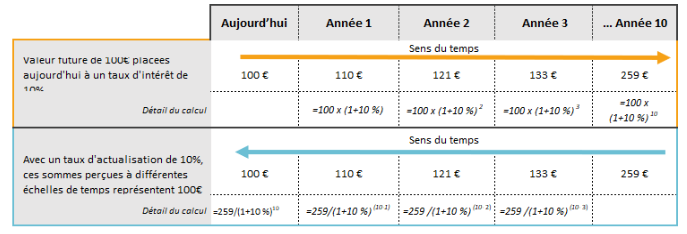
The interest rate is used to determine the future value of a present amount: €100 invested at 10% will be worth €110 in one year and €259 in 10 years.
The discount rate allows us to do the opposite: with a discount rate of 10% per year, €110 received in one year’s time has a present value of €100. The same applies to €259 received in ten years’ time.
Please note: the above reasoning is based on the assumption that there is no inflation. This is generally the framework within which economists reason. The income levels shown in the table are calculated on the basis of the price level in the starting year.
A high discount rate “crushes” the future
Let’s note a fundamental point right away: the higher the discount rate, the lower the present value of future amounts.
Present value of future €100 using different discount rates
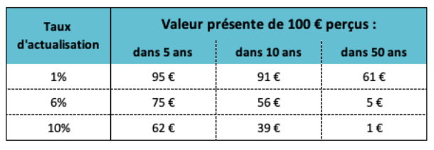
As you can see from this table, with a 10% discount rate, €100 received in 50 years is “worth” €1 today. With a discount rate of 1%, the same future €100 would be worth €61 today.
As we shall see in the following sections, the discount rate is decisive in deciding whether or not to invest, whether in the private or public sector. In short, it determines how much you’re willing to invest today to receive tomorrow.
In the table above, an investor is prepared to contribute €61 today to a project that will earn €100 in 50 years’ time at a discount rate of 1%, but only €5 at a rate of 6%.
For now, let’s remember that the higher the discount rate, the less the future counts in today’s calculations.
This is important when it comes to investment typology: with a high discount rate, a project that generates income in the short term will appear much more interesting than one that generates income in the longer term.
This is also important in ecological terms. On the one hand, ecological projects often have long-term “returns”. On the other hand, many projects generate costs at the end of their life (dismantling a factory, nuclear or coal-fired power plant, soil decontamination, reclamation of a mining site, etc.). With a high discount rate, these expenses, which will occur in the future (often several decades), count for very little in the initial calculations aimed at assessing the profitability of the investment in order to decide whether or not to go ahead with it.
We’ll now go into more detail about the different types of players who use discounting to make economic calculations.
The discount rate: a key factor in private investments
A company looking to renew its equipment or develop new activities needs to invest. To determine whether this investment is financially worthwhile, the company’s management calculates the return, using a discounting technique. A financial player hesitating between two types of investment (for example, investing in the capital of an industrial company or in a real estate project) will act in the same way.
The internal rate of return (IRR) is the discount rate used to evaluate the profitability of an investment
One of the methods frequently used to assess the return on an investment is to compare the cost of the initial investment with the present value (i.e. the discounted value) of all future cash flows. 1 that will be generated by this investment over its lifetime.
To do this, we use the net present value (NPV), which takes into account the cost of the initial investment as a negative and the future income streams (once expenses have been deducted) as a positive. Since the latter occur at different timescales, they need to be discounted. But how do you determine the right discount rate?
By convention, investors use the internal rate of return (IRR): this is the discount rate that reduces the NPV to 0.
Let’s look at a numerical example for a better understanding.
Example – NPV and IRR of The Mainstream Economy investment project
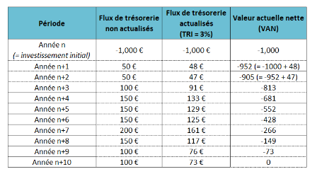
The Mainstream Economy invests €1,000 to purchase machines with a three-year lifespan, and expects to generate the following revenues.
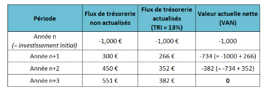
The project’s Internal Rate of Return, i.e. the rate at which the initial investment of €1,000 is offset by discounted future income, is 13%.
An investment is considered financially profitable when the IRR exceeds the cost of financing (WACC)
The cost of financing the company (or project) is calculated according to :
- the financial structure of the company (or of the specific investment project), i.e. the breakdown between equity (capital) and debt;
- the respective costs of capital and debt.
Note that the term commonly used is not “cost of financing” but “weighted average cost of capital”. 2 which is confusing, since financing can be based on both capital and debt.
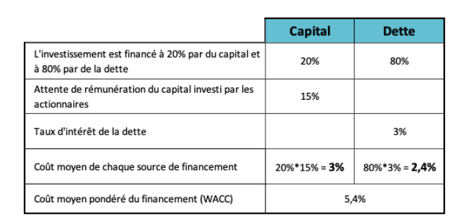
Example of WACC calculation for The Mainstream Economy investment project
The company financed its investment with 80% debt (negotiated with the bank at an interest rate of 3%) and 20% equity (with an expected return of 15%). The WACC is therefore 5.4%, well below the IRR of 13% mentioned above. The project developed by The Mainstream Economy is therefore highly profitable!
In “normal” financial practice (as taught in business schools), a financial investor should aim to achieve an IRR equal to or greater than the weighted average cost of capital, i.e. a zero or positive NPV.
When the NPV is positive, we say that the company or project “creates value”, which is highly debatable, since in this case it’s only a question of financial gains for investors.
To continue our previous example, The Mainstream Economy’s investment project will create annual “value” of 7.6% (13%-5.4%) multiplied by the size of the investment.
Financial backers’ remuneration requirements
In the case of debt, the interest rate is negotiated between the lender (a bank or bond investor) and the company’s management. These rates depend on various factors relating to the lenders’ perception of risk (the company’s financial situation, its sector of activity, its competitive positioning, the economics of the project itself), as well as the general level of interest rates. This last point is particularly important: very low very low interest rates of the 2010 decade have kept financing costs down across the board.
With regard to equity investors, i.e. shareholders, we can distinguish two cases. For a listed company, the expected return on equity (ROE 3 ) is broadly defined by “the market” and by the company’s competitive position in its sector. It should be pointed out here that “the market” is not an abstract entity, but a place of confrontation and balance of power, which can change as a result of the relative powers of the various players and institutional arrangements. ROE has increased overall since the 1950s, notably as a result of the acceleration of “globalization” and the financialization of the economy in the 1980s. For an unlisted company, shareholders have more latitude when it comes to ROE.
As a general rule, capital investors’ expectations are as high as possible: with many investment options to choose from, they target those that promise the highest returns. What’s more, these investors are often intermediaries who manage the savings of clients to whom they have promised a return.
The cost of financing, and therefore the returns expected from financiers, influence the type of project, putting long-term projects at a particular disadvantage.
Indeed, a high WACC implies a high IRR too, otherwise the project will not be considered profitable and will not find financing.
As we saw in Part 1, the higher the discount rate (in this case, the IRR), the less future income counts. Projects that generate income over the long term are therefore at a disadvantage compared with those that promise income in the short term.
For example, let’s imagine that The Other Economy (TOE) wants to develop a project whose initial cost is also €1,000, but whose future revenues are lower and more spread out over time than those of TME.
Example – NPV and IRR of The Other Economy’s investment project
The IRR is therefore lower (around 3%). With the same financing cost as The Mainstream Economy project (5.4%), the investment is considered unprofitable and unlikely to find private financing.
This is the case for many ecological transition projects, whose ecological and social benefits are generally not 4 in financial calculations.
Let’s take the example of a steel plant that needs to change its production methods to make them more environmentally friendly. This requires heavy investment to set up the new plant processes. The end product remains the same, but has simply cost more to produce because of the initial investment. Consumers are therefore unlikely to pay more for the new steel. If the company raises the price of its new steel too much, consumers will turn away from the company, and it will not earn enough money to repay the initial investment. The benefits of such an operation are rather small for the company, even though they benefit society as a whole through reduced pollution (ecological and social benefits). However, these benefits are not taken into account in the company’s calculations.
If financiers perceive the project as risky (e.g. because it’s a new product, and/or in an uncertain regulatory environment), their return expectations can’t be met, and the project won’t go ahead for lack of financing.
To overcome this difficulty (which prevents some of the transition projects from being financed), several solutions are conceivable and have been partly implemented.
- patient capital”, i.e. investors willing to accept lower returns, or public financing. As capital investors, the State and public structures do not have the same expectations of financial return as most private investors (for the reasons developed in part 3).
- improve the operational profitability of the project through public measures (such as various forms of public aid and subsidies, feed-in tariffs, payment for ecosystem services).
- reduce the cost of financing through public schemes (guarantees, interest-rate subsidies, partial financing, etc.).
The discount rate is also common public data
As an investor, the State does not seek the same type of profitability as a private player.
Every year, the French state and local authorities invest in a wide range of projects: infrastructure, energy production, public transport, public buildings and more. In 2021, according to the French Ministry of the Economy, public investment totaled 89.7 billion euros. 5 or 3.7% of French GDP.
These investments obey different profitability logics from those of the private sector. Their primary objective is not to make money for the state, but to bring economic, social or ecological benefits to the community. And they are expected to achieve these objectives at the lowest possible “cost” to the taxpayer.
This involves calculating the “socio-economic return” on public investment. One of the tools used to do this is socio-economic evaluation, also known as cost-benefit analysis (CBA).
CBA consists in comparing the costs and benefits of a project in a monetized balance sheet, integrating not only the financial aspects but also the non-monetary impacts (time savings for transport users, safety, access to public services, reduced pollution, greenhouse gas emissions, etc.). As these costs and benefits are spread over several years, these calculations involve a discount rate.
In France, for example, 40.4% of the projects under study, listed in the in the 2022 inventory of the Secrétariat Général pour l’Investissement have undergone a CBA. It should be noted that these assessments are not carried out for all projects (in particular, there are financial thresholds), are supplemented by other types of assessment (e.g. non-monetized environmental assessments) and do not have decision-making value (a negative result does not necessarily lead to the abandonment of a project).
Choosing the right discount rate for an investment project is a highly sensitive issue.
We’ll see in another section that CBA is in itself a highly debatable method for many reasons. Here, we limit ourselves to showing the key role of the discount rate in these calculations.
For public investments, the discount rate to be applied to projects is determined conventionally by the public authorities, following recommendations by commissions of economists.
As with private investments, its level has a major influence on the CBA result of any project with a lifespan of several decades, which is the case for most infrastructure projects.
Take the example of a nuclear power plant. Its construction represents a major investment over several years. Profits from the sale of electricity follow. They are more modest, but last for the entire life of the plant (several decades). In this type of project, the CBA is very sensitive to the discount rate used. If the rate is high, the benefits quickly count for almost nothing, and the project does not appear profitable. If the rate is lower, the discounted sum of benefits may exceed the initial cost, and the project considered profitable can be launched. Finally, if the discount rate is very low, and the end-of-life of the plant entails significant costs (dismantling, very long-term waste management), the project may once again be downgraded. Things get even more complicated when we add non-market costs and benefits (avoided CO2 emissions, environmental impacts in terms of water abstraction or waste management, etc.).
It’s easy to see how the choice of discount rate can give rise to multiple controversies: the use of a high or low rate being of strategic interest to the detractors or, on the contrary, the promoters of a project.
“Controversies on this subject arise for all types of major projects: waterway developments in the USA in the 1950s, construction of nuclear power plants, conservation of natural resources. As economists do not agree among themselves on the choice of discount rate, or even on a reasonable narrow range, arguments are perpetually raised one way or the other. The controversy over major infrastructure projects becomes a controversy over discounting, and this in turn feeds the controversy over the initial project.” Antonin Pottier.
Ramsey’s rule is one of the main methods used by economists to determine the discount rate.
Given its importance in determining the “socio-economic profitability” of a public investment, the discount rate is a public datum whose determination is a political issue.
This has greatly boosted academic research on the subject, as Groom and Hepburn show in an article published in 2017 6 in which they highlight the double positive interaction between political interest in updating and academic research on the subject. Their study is based on data from the UK, USA, France and the Netherlands, between 2002 and 2017.
This academic interest is matched by a highly operational scope. Indeed, as we shall see in the next section, using France as an example, the discount rate for public investment projects is set by commissions with an official mandate to do so. These commissions are headed by and/or call on the services of economists. It is therefore important to understand the methods they use.
Here, we describe Ramsey’s rule, which is the most commonly used. In part 4, we’ll use the example of global warming to show just how open to criticism this rule is.
The Ramsey rule
Economists working on discount rates generally adopt a theoretical approach, different from the financial practice described in Part 2.
It consists in reasoning from the consumer’s point of view, and determining the conditions that enable him to maximize his intertemporal utility (consumption). They generally adopt a formula known as “Ramsey’s rule”. 7 which breaks down the discount rate into “ethical” and “political” parameters.
In its simplest form, this formula can be written as follows: ???? = p + n x ????
With :
???? = discount rate
p = the rate of pure preference for the present (also known as TPPP)
This term reflects the idea that individuals would prefer to consume today rather than tomorrow, either for psychological reasons (impatience), or because of uncertainty about the future (there is a non-zero probability of dying before receiving future income).
n = time inequality aversion (or intertemporal consumption elasticity).
This term reflects people’s preference for “smooth” consumption over time. For example, you might prefer to spend your whole life on €2,000 a month, rather than spending the first half on €500 and the second half on €3,500. The larger this term, the more it reflects a desire for consumption (and therefore income) that is smooth over time. The smaller the term, the greater the tolerance for heterogeneous consumption. In short, it gives priority (to a greater or lesser extent) to the poorest period.
???? expected income growth rate (similar to GDP growth rate)
The parameter n is multiplied by the growth rate. The idea is as follows: if I have more income in the future than I have today, I will tend to give more weight to my present income (and all the more so as my aversion to intertemporal inequality is strong). Conversely, if my income is decreasing, I will give more weight to future income. It should be noted that in Ramsey’s formula, this reasoning is extended to all economic agents considered globally (it therefore takes no account of the unequal distribution of growth between individuals).
Introducing the notion of risk into the Ramsey formula
This initial formula was later made more complex to include a risk premium. Without going into the equations (which may vary depending on the model used), it should be noted that the notion of risk is considered in a rather limited way: the aim is to evaluate the risks borne by the project itself (and not those it avoids, for example), in particular its dependence on economic growth.
Let’s take an example. We start with the risk-free discount rate (Ramsey formula) and add a risk premium according to the project’s estimated dependence on future economic growth. If this premium is positive (e.g. trains are less frequented when economic growth slows), the risk discount rate is higher than the risk-free rate. Conversely, if the risk premium is negative (e.g. hospital use is higher when the economy is struggling), the risk discount rate is lower than the risk-free rate.
What do official reports on the subject recommend in France?
As explained in the previous section, the choice of discount rate for public investment projects is a highly sensitive issue.
In France, administrative doctrine in this area has been established by commissions, mandated by forward-looking bodies attached to the Prime Minister. 8 . It has evolved considerably over the last few decades.
While the discount rate had been set at 8% in 1985 by the Commissariat Général du Plan, until the early 2000s, the Lebègue report (2005) 9 proposed lowering the rate to 4% for the first 30 years following investment in a project, and then gradually decreasing it over the life of the project to a minimum value of 2%.
It was completed in 2011 by the Gollier report 10 which proposed the introduction of a risk premium, increasing the discount rate if the project is exposed to macro-economic risks (such as a loss of economic growth), and decreasing it in the opposite case. This idea was further developed in the Quinet report report in 2013 11 .
Prior to 2021, the risk-free discount rate used in France was around 2.5%, in line with the average for other OECD countries. The book Cost Benefit Analysis and the Environment by Atkinson, Braathen, Groom and Mourato, commissioned by the OECD, summarizes in chapter 8 the main discounting approaches adopted by member countries.
Discounting recommendations in several OECD countries
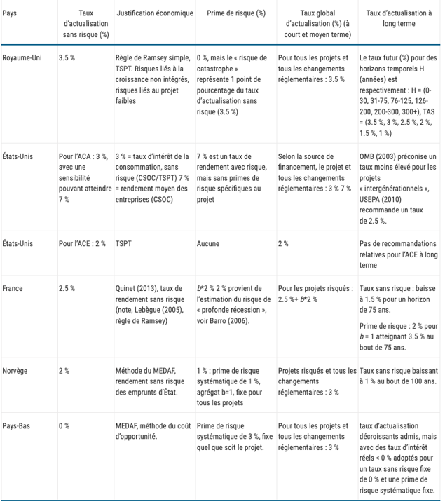
Source Cost-benefit analysis and environment (OECD, 2019), Table 8.5
In 2021, a group of experts working for France Stratégie 12 proposed a proposed a new method for determining the discount rate taking into account the project’s risks (linked to its dependence on economic growth). The risk-free rate is now 1.2%.
As we have seen, determining the discount rate has a very real impact on assessing the profitability of public investment projects. However, the methods used, presented as scientific, suffer from numerous shortcomings. This is what we’ll see in the next section, using the famous example of global warming.
The discount rate and assessing the long-term economic impacts of climate change
The emergence of climate issues has led some economists to attempt toassess the long-term impact of global warming on GDP. The debates and controversies that have taken place highlight several important points about the discount rate:
- As we have already seen, depending on the discount rate chosen, the long-term impacts of climate disruption will carry more or less weight. It is therefore a decisive parameter for the results of the analysis and the resulting recommendations.
- This choice necessarily involves ethical and ideological reflection. It cannot be left to the technical debates of economists alone.
This section includes many of the elements of Antonin Pottier’s analysis in his book Comment les économistes réchauffent le climat.
The use of the discount rate in economic calculations relating to the fight against climate change
In 2018, economist William Nordhaus was awarded the Nobel Prize in Economics for “his pioneering work on the integration of climate change into long-term macroeconomic analysis”. In the early 1990s, he designedthe DICE macroeconomic model, which combines a long-term growth module with a climate module.
Nordhaus’ aim is to use this model to determine the economically “optimal” trajectory for greenhouse gas emissions (and hence warming), with a view to maximizing intergenerational “well-being” (equated with consumption). If the world follows this trajectory, the current costs of combating global warming will be offset by future benefits (i.e. avoided damage). The aim is also to deduce recommendations in terms of public policy, and in particular to put a price on CO2, the main (but not the only) greenhouse gas responsible for global warming. 13 .
This model therefore performs a cost-benefit analysis, with on the one hand the costs generated by the implementation of policies to combat climate change (renewable and nuclear power generation, building insulation, electrification of transport, introduction of soft mobility solutions, agricultural transition, etc.), and on the other the benefits, i.e. the damage linked to climate disruption that these policies will make it possible to avoid.
This type of approach poses a number of problems.
- The objective itself raises questions: the fight against climate change is much more about preserving the habitability of our planet for human beings than it is about maximizing consumption over time.
- The level of climate policy costs (known as abatement costs) is also controversial (some of these policies will create activity and are therefore not costs at the macro-economic level).
- The future damage caused by global warming is obviously extremely difficult (and, in any case, impossible) to estimate, given the many physical, temporal, geographical and social uncertainties involved. In the Global warming: what impact on growth? we explain in detail the extent to which the methods used by economists to assess these damages are questionable, and lead to an underestimation of the impact of global warming on the economy.
Finally, given that this is an intertemporal analysis, the question of the discount rate obviously arises. As we have seen, the higher the discount rate chosen, the more the future is crushed in relation to the present. As a result, the weight of the future benefits of “climate” investments (i.e. avoided climate damage) will weigh very little in the balance of the cost-benefit analysis.
Depending on the discount rate chosen for the modelling, the recommendations that emerge from the analysis may therefore discourage the investments needed to avoid too much warming, since these never appear to be profitable.
This is what we’ll see when we summarize one of the most famous controversies surrounding the discount rate in the following section.
The controversy over the economic impact of global warming
Although Norhdaus began his work on macroeconomic climate modeling in the late 1970s, the results of the first completed version of his DICE model were published in 1994 in his book “Managing the Global Commons”. In it, the cost-benefit analysis carried out led to the recommendation of an (economically) “optimal” CO2 emission trajectory leading to an atmospheric CO2 concentration of 650 ppm. 14 more than twice the pre-industrial concentration. Its recommendations for combating global warming are consequently rather limited.
Episode 1: Nordhaus / Cline
At that time, William Cline, a lesser-known economist, had already published a similar analysis. 15 but he advocated far greater emission reductions.
Yet both economists used the same analytical framework and relatively similar parameters. The main difference lies in the discount rate used: 6% for Nordhaus and 1.5% for Cline.
Comparison of the parameters chosen by Nordhaus and Cline to calculate the discount rate (using Ramsey’s rule)
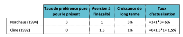
In his book, Nordhaus strongly criticizes Cline’s choices on the grounds that they reflect a philosophical stance far removed from the “positive” (neutral) attitude an economist should adopt. Indeed, Cline justified his choice of a pure present preference rate (PPPR) of 0% by the fact that it seemed ethically indefensible to him to give more weight to present generations than to future ones. He would therefore have set the discount rate on the basis of his beliefs rather than facts. 16
Episode 2: Nordhaus / Stern
Twelve years later, the controversy resurfaces, but this time with much more fanfare. Nicolas Stern, a renowned economist, head of the British government’s economics department and former chief economist of the World Bank, adopts a position close to Cline’s. His report on the economics of climate change is a good example of this. His report on the economics of climate change (2006) 17 submitted to HM Treasury in 2006, attracted considerable media attention.
This is the first time that the fact that global warming could have major negative economic consequences has been massively publicized in the press and among decision-makers, and that it is therefore necessary to reduce greenhouse gas emissions rapidly and significantly.
Of the many issues raised in the 600-plus pages of the report, it is the discount rate that attracts the most attention from economists. It’s also on this point that they focus their criticisms.
Here again, economists criticize him for not relying on market rates and for letting himself be guided by his own “opinion” of climate change. Nordhaus accuses him, for example, of proclaiming himself, through his choice of low discount rates, “a global social planner… fanning the dying embers of the British empire.” 20 .
Let’s not forget that the disastrous consequences of global warming on the planet’s habitability are not an “opinion” but a scientific consensus among climatologists.
These seemingly technical debates are not neutral.
While climate inaction cannot of course be attributed to the recommendations of economists alone, the fact remains that the rhetoric of figures like Nordhaus has contributed to it. For almost 15 years, the message that global warming would have no significant impact on GDP in the long term dominated among political decision-makers. As you can see from the table below, depending on the discount rate used, the level of benefits to be expected (climate damage avoided) from a climate investment is not at all the same. So there’s no need to implement over-ambitious climate policies. Nordhaus has long advocated very gradual climate policies, starting with low emission reductions and building up over the course of the 21st century. The Kyoto Protocol, for example, was too ambitious in his eyes.
Effects of different discount rates on the amount of avoided damage needed to make €1,000 invested today in climate policies profitable.
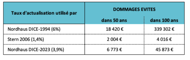
In the first version of DICE (1994), €339,000 of GDP loss over 100 years must be avoided to justify €1,000 of investment today. This is almost 85 times more than using Stern’s discount rate. Note that in the latest version of DICE (2023), despite all the advances in climate science, the rate used by Nordhaus remains very high.
Let’s take another example.
This one is deliberately extreme, and slightly inspired by the film Don’t Look Up.
Suppose :
-global GDP, currently around 93,000 billion USD, will grow by 2% every year, reaching 673,000 billion in 100 years’ time.
-astrophysicists predict that in 100 years a comet will hit the Earth and destroy the entire economy (not to mention humans). GDP in 100 years and 1 day = 0, for an infinite duration.
With a discount rate of 6%, how much would present generations be willing to invest to build the machine needed to destroy this comet?
Answer: a maximum of 52,000 billion, or barely 50% of current GDP, to avoid the end of humanity!
The choice of discount rate is inevitably ideological
The main argument put forward by Cline’s and Stern’s detractors is that they adopt a philosophical, not a scientific, stance. Yet on closer examination, their approach is no less so.
The discount rate incorporates two parameters by which the present counts for more than the future
The first is obvious: the pure present preference rate (PPPR).
The second is the economy’s growth rate, which is assumed to be positive in almost all models. The future is therefore considered, by construction, to be richer than the present. The growth rate being combined with the aversion to intertemporal inequality (which values the poorest period), the result is a positive discount rate, even if the TPPP is zero.
But this assumption of an eternally positive growth rate in itself raises questions. 21 . Without getting into the debate about the impact on growth of implementing a genuine ecological bifurcation, the health crisis, the energy crisis, the first effects of climate disruption and the collapse of biodiversity all legitimately raise the question of the possible or even probable future decline in GDP.
Is the relationship between individuals and the future limited to the rate of preference for the present?
Ramsey’s rule reduces individuals’ preferences for the future to the single parameter of TPPP, which reflects a form of human impatience. As Antonin Pottier notes, this conception only came into play in the second half of the 20th century. “Before that, economists had a richer conceptualization of the relationship to the future, their reasoning incorporating motives of legacy, uncertainty, self-constraint.” 22
Even limiting itself to reflecting this impatience, this decision model doesn’t capture reality. For example, if a person prefers to receive a euro today rather than tomorrow (which shows a preference for the present), then he or she is supposed to prefer to receive a euro in a year’s time rather than in a year and a day’s time, when in general he or she makes no difference between the two possibilities.
Is it really possible to deduce the individual preferences of economic agents (summarized by the parameters p and n) from the interest rates observed on the markets?
While Ramsey’s formula provides a theoretical framework for reflection, it is not directly operational. Neither the rate of pure preference for the present, nor aversion to temporal inequality are observable: they are unknown parameters. As Antonin Pottier explains, to make the tool operational, economists will set the discount rate to be equal to the interest rate in the economy.
Here’s the justification “Let’s suppose that an economic agent’s discount rate (let’s say a = 2%) is lower than the interest rate (r = 5%): this agent then has an interest in investing his available funds today and consuming them tomorrow: €100 invested will yield €105 tomorrow. For the agent, this money consumed tomorrow is equivalent to consumption today of 105 / (1 + a) = 105 / 1.02 ≃ 103 (the discount rate reduces future values (here the €105) to the equivalent of present consumption). This equivalent of €103 is greater than the one hundred euros of consumption the agent can obtain by spending this sum today. The agent, less “impatient” than the rest of the economy, therefore seeks to save in order to transmit wealth in the future. The arrival of the savings the agent wishes to invest reduces the interest rate. Equilibrium is reached when the interest rate equals the discount rate for all agents: agents then no longer want to modify their decisions to save funds.” 23
Such reasoning is only possible in an extremely theoretical context: the agents’ preferences are all identical (they want to maximize their intertemporal consumption), they are rational, they have no constraints on borrowing, all information is available, prices transcribe individual wills and owe nothing to the irregularity of transactions, the weight of fortunes, the excitement of gambling, and so on.
Of course, these conditions are never met. In reality, interest rates (which vary according to the “financial instruments” we’re talking about) reflect market frictions, not agents’ expectations of the future, nor an ideal convergence on a market that doesn’t function as in theoretical models. The argument for deducing discount rates from market rates is therefore unfounded.
Collective decisions are different from individual decisions
The aim of cost-benefit analyses is to inform public action, whether it be the choice of an investment or the decisions to be taken to combat climate change. The nature of the decisions to be taken is therefore very different from that which would be taken by a company or an individual. On the one hand, we have the decision of a private agent involving his own future (that of his company, the assets of a household); on the other, the decision of a State or territory involving the entire community it administers today and in the future.
But in the logic of Ramsey’s formula, the collective decision must derive from individual preferences, as expressed by economic choices and visible on the markets via interest rates. As Antonin Pottier notes, this is a “particular conception of collective decision-making, which has no more legitimacy than any other. Of course, collective decision-making must have some connection with individual choices, at least in a democratic society. It is precisely the role of democracy to institute procedures that enable collective decisions to be forged from individual opinions. Recourse to the market is one possible procedure, but there is no proof that it is the only or the best, the most moral or the fairest.”
Let’s take the case of TPPP. At the consumer level, we can understand why economists assign it a positive value: consumers may be impatient, or at least wish to benefit from their consumption in the present rather than in a year’s time, given their non-zero risk of dying within a year. On a macro-economic scale, the choice of a positive TPPP raises more questions. It means openly giving future generations less weight in the decision, which raises serious questions of ethics and intergenerational equity. This is why, as we have seen, some economists such as Cline and Stern are in favor of a TPPP close to 0. It is therefore an ideological choice, in the sense of a societal choice. This is also the approach adopted by the economists who contributed to the latest IPCC report.
We conclude that a broad consensus is for a zero or near-zero pure rate of time preference for the present
This choice is no more ideological than basing the discount rate on the postulate that collective preferences are equal to the sum of individual preferences, that the latter are guided by the desire to maximize consumption over time, and that this is correctly reflected in interest rates observable on markets.
Whatever the justifications adopted, the choice of discount rate remains a choice in the full sense of the term.
Conclusion
The choice of discount rate is of decisive importance for all long-term projects, and therefore for ecological transition projects. In the private sector, this choice is highly dependent on the cost of financing and, more generally, on the expected return on capital: favoring long-term projects therefore implies acting at this level. In the public sector, it’s a matter for the administration to decide, so the room for manoeuvre seems, on the face of it, greater. Presented as technical and neutral, the determination of the discount rate is in reality a choice in the full sense of the term, which is much more a matter of collective deliberation than expert debate. As a result, there is a wealth of literature and positions on the subject, and no single proposed method allows us to reach a consensus. As Gaël Giraud puts it: “There is no such thing as a [discount rate]. 24 “and its choice is a matter of pure convention. In choosing this metaphysical variable, many economists are basically choosing their response to ecological problems. 25 .
- It should be pointed out that this refers to cash flows, i.e. cash inflows minus cash outflows (and not to book profits or other profit indicators which would not be in cash, as they cannot be invested). ↩︎
- or WACC for “Weighted Average Cost of Capital”. The English term is commonly used. ↩︎
- Return on equity ↩︎
- This is done indirectly via environmental taxes or CO2 quota markets, which increase the cost of pollution-generating projects, but rarely enough to make them unprofitable. What’s more, the majority of ecological and social benefits are not recognized in corporate accounts (see the module on corporate accounting). ↩︎
- See the report: Evaluation of major public investment projects, appendix to the 2023 Finance Bill. ↩︎
- Reflections-Looking Back at Social Discounting Policy: The Influence of Papers, Presentations, Political Preconditions, and Personalities, Groom, B; Hepburn, C, 2017, Review of Environmental Economics and Policy ↩︎
- Named after Ramsey’s contribution, F. P. A Mathematical Theory of Saving, The Economic Journal, (1928), Ramsey’s rule actually dates back to the optimal growth theories of the 1960s. ↩︎
- Successively the Commissariat général du Plan, the Centre d’analyse stratégique, the Commissariat général à la stratégie et à la prospective and France Stratégie. ↩︎
- Commissariat général du plan (2005), Le prix du temps et la décision publique. Révision du taux d’actualisation public, report by the group of experts chaired by Daniel Lebègue, Paris, La Documentation française. ↩︎
- Center d’analyse stratégique (2011), Le Calcul du risque dans les investissements publics, report by the mission chaired by Christian Gollier. ↩︎
- Commissariat général à la stratégie et à la prospective (2013), L’Évaluation socioéconomique des investissements publics, rapport de la mission présidée par Émile Quinet. Volume 1 and Volume 2 ↩︎
- France Stratégie (2021), Révision du taux d’actualisation, Complément 1 au Guide de l’évaluation socio-économique des investissements publics. ↩︎
- To find out more about why economists recommend putting a price on CO2, see ” To solve the problem of pollution, all you have to do is put a price on it “. ↩︎
- Annual CO2 emissions increase the atmospheric concentration of this gas, which is measured in parts per million (ppm). Find out more in our Measuring GHGs fact sheet. The pre-industrial concentration of CO2 was 275 ppm. The “economically optimal” trajectory of CO2 emissions recommended by Nordhaus therefore leads to a more than doubling of atmospheric concentration. Note that in 2023 the analysis has not changed significantly, since in DICE2023 the optimal trajectory leads to an atmospheric concentration of 600 ppm in 2100 (and a warming of +2.73°C). ↩︎
- Cline, William R. (1992) – Global Warming: The Economic Stakes, Institute for International Economics. ↩︎
- For Nordhaus, the facts are the interest rates observed on the markets (we explain why in section 4.3). In reality, Cline did indeed conform to current practice: the discount rate he arrived at was close to the yields on US Treasury bonds (around 1.5% at the time), whereas Nordhaus based his calculations on the higher yields on certain financial securities. ↩︎
- See Stern, N. H. (2006), Stern Review: The Economics of Climate Change, Volume 30, London: HM treasury. ↩︎
- See Dasgupta, P. The Stern Review’s Economics of Climate Change, National Institute Economic Review 2007; Nordhaus, W. D. A Review of the “Stern Review on the Economics of Climate Change, Journal of Economic Literature, 2007; Weitzman M. L. A review of the “Stern Review on the Economics of Climate Change”, Journal of Economic Literature, 2007; Mendelsohn R. Is the Stern Review an Economic Analysis?, Review of Environmental Economics and Policy, 2008; Yohe, G. W. and Tol, R. The Stern Review: Implications for Climate Change, Environment: Science and Policy for Sustainable Development 2007. ↩︎
- However, he chose a rate of 0.1% rather than 0 because of the minute probability of humanity disappearing each year, which leads to a slight preference for the present. ↩︎
- A Question of Balance: Weighing the Options on Global Warming Policies (2008) ↩︎
- To find out more, see Can there be growth without energy? and Global warming: what impact on growth? ↩︎
- See Pottier page 250. Further information Frederick, S. Loewenstein, G. and O’Donoghue, T. (2002) Time Discounting and Time Preference: A Critical Review Journal of Economic Literature. ↩︎
- How are economists warming the planet? pages (174-175) ↩︎
- Gaël Giraud uses the term “discount rate” to designate the discount rate. ↩︎
- Gaël Giraud, Les modèles économiques et financiers face à la polycrise écologique, April 2021, Annales des Mines : https://www.annales.org/re/2021/re102/2021-04-03.pdf ↩︎