
This text has been translated by a machine and has not been reviewed by a human yet. Apologies for any errors or approximations – do not hesitate to send us a message if you spot some!
Interest rates are a central component of our economies and financial systems. Households, companies and governments borrow from banks and/or financial markets. Interest rates are an important parameter in their investment decisions, and the resulting financial burdens can weigh heavily on their economic health. Understanding how these rates are formed and knowing how to anticipate them is therefore an essential challenge in financial economics.
This fact sheet first explains the importance of interest rates for the real economy. Next, we present the Taylor rule, a theoretical economic framework for modeling central bank policy rates. We also look at a concept central to interest rates: the yield curve, which compares short- and long-term rates. Finally, we look at the dynamics of long-term interest rates and the factors that can influence them.
The importance of interest rates for households, industry and the ecological transition
The spectacular rise in key rates at the European Central Bank (ECB) – and also at the Fed (US central bank) – in early 2022 followed a prolonged period of near-zero or even negative key rates in the 2010s.
Key European Central Bank interest rates between 2009 and 2024
Reading: In 2010, the ECB’s main refinancing rate was 1%, the marginal lending rate was 1.75%, and the deposit facility rate was 0.25%.
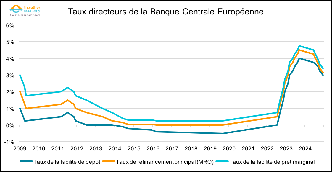
Source Key ECB interest rates, European Central Bank. Accessed on 21/12/2024.
Note: The ECB has three key rates.
The Main Refinancing Operations (MRO) rate: this is the rate at which commercial banks can borrow money from the ECB for a period of one week.
The marginal lending rate: this is the rate at which banks can borrow funds from the ECB overnight.
The deposit rate: this is the rate at which banks can deposit their surplus cash with the ECB overnight.
Central bank key rates are short-term borrowing rates. Commercial banks borrow from their central bank at these rates 1 . These key rates are used by central banks as their main tool for 2 to achieve their inflation targets – inflation control (or “price stability”) being the primary mandate of the largest central banks today.
Indeed, according to the quantitative theory of money, high inflation is always the result of too much money in circulation. While money creation can have an effect on inflation, it is clearly not the only cause of rising prices. We discuss the criticisms and flaws of the quantitative theory of money in our Inflation and Money fact sheet.
In any case, it is within this neoclassical framework that central banks use key rates with the following ambition: an increase in key rates should, in theory, lower inflation – while a decrease in rates should, on the contrary, raise inflation.
Although central bank key rates may seem abstract, they play a cardinal role in determining the rates at which households and businesses can borrow in the medium and long term (as we’ll see throughout this factsheet). The episode of rising key rates in 2022 clearly illustrates that a sharp increase in key rates leads to a rise in borrowing rates for households, particularly for mortgages. This deprived many households of access to home ownership – due to reduced borrowing capacity – and ultimately reduced overall demand for home loans.
Household borrowing capacity is affected by key interest rates
Reading: In October 2024, the average rate for home loans to individuals living in France was 3.46%, and the monthly value of corresponding loans was around half that of January 2020.
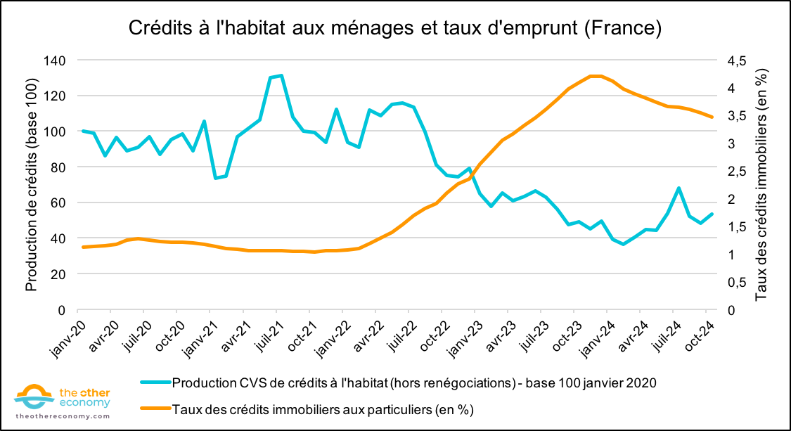
Source Banque de France, Observatoire Crédit Logement/CSA.
Note: CVS stands for Correction of Seasonal Variations .
In particular, long-term rates represent a fundamental challenge for the ecological transition, which requires heavy investment over several decades. 4 Investments in the ecological and energy transitions are therefore significantly impacted by high long-term interest rates. 5 Indeed, as the graph below illustrates, investments in solar and wind power are more capital-intensive than investments in gas or oil. In other words, investing in renewable energies requires higher initial capital than fossil fuels. On the other hand, oil and gas projects generally have higher post-deployment operating costs than wind or solar projects.
A direct consequence of this is that investments in green energies are much more sensitive to a rise in rates than investments in more carbon-intensive energies.
Many economists, countries and associations (including France in 2023) have also expressed their support for the introduction of a green interest rate. 6 This green rate would be an advantageous rate at which banks could refinance themselves, provided they financed “green” projects (as defined by the European taxonomy). Find out more by reading the Proposal Lowering the cost of ecological transition with a green interest rate from the ECB .
Wind and solar power are particularly capital-intensive
Reading: For offshore wind power, initial investments (CAPEX) account for around 66% of total project investments (i.e., initial investments plus operating costs – CAPEX and OPEX). The most capital-intensive technologies are thus on the left-hand side of the chart.
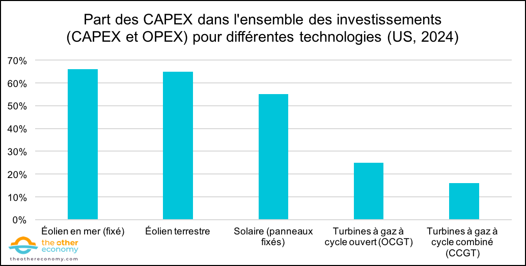
Source Peter Martin, et al, Conflicts of interest: the cost of investing in the energy transition in a high interest-rate era, Wood Mackenzie, 2024.
Note: These estimates apply to the United States in 2024. They assume that projects are 55% debt-financed over 15 years.
The Taylor rule: a model for better understanding central bank key rates
As we’ve just seen, central bank interest rates play a cardinal role in our economies – whether for governments, households or businesses. So it’s natural to ask: how are these rates determined by central banks? How can we model them?
The Taylor rule is the benchmark rule for modeling central bank policy rates. Its formulation links key rates to “known” data: inflation and Gross Domestic Product (GDP). 7 This rule is often cited in the literature on central banking, and is used to explain the behavior of central banks when they raise or lower rates. 8 Following this rule is thus linked to the following three ideas (ideas often taken for granted, but which can be discussed):
- inflation is the central bank’s priority;
- the central bank is the institution responsible for controlling inflation;
- Acting on interest rates is the most effective way for a central bank to fight inflation.9
The first two ideas are, moreover, incorporated into the European treaties which define the Central Bank’s mandate ( art. 127 TFEU ).
The Taylor rule, initially a descriptive tool, has gradually taken on a more prescriptive role for monetary authorities.
The Taylor Rule aims to define a guideline for monetary authorities.
Origins of the Taylor rule
The Taylor rule, first formulated by economist John B. Taylor in 1993 10 and popularized by a Goldman Sachs study in 1996, is now a benchmark tool, often used by the OECD and cited by several central banks. It is used to define a short-term key rate, known as the Taylor rate, which, according to neoclassical economic theory, would enable the central bank to achieve its price stability objective (2% inflation in the case of the ECB or the Fed). 11
This rate is based primarily on three elements: the central bank’s inflation target, current observed inflation, and theoutput gap – the gap between the economy’s actual output and its potential output (more details in part 2.3).
First limits identified by Taylor in 1993
Before going into more detail on the Taylor rule, it’s worth noting that Taylor himself, in 1993, doesn’t see it as a prescriptive rule to be followed meticulously. Indeed, he already lists some notable limitations (which we develop in part 2.3).
To support his point, he uses, among others, the case of the 1990 oil shock (which followed Iraq’s invasion of Kuwait). 12 . Following this event, soaring oil prices (which doubled in the space of a few months) led to high inflation in the United States, which, according to the Taylor rule, would imply a substantial increase in Fed policy rates.
However, Taylor argues that, once it becomes clear that the price rise is temporary – in this case, due to a geopolitical crisis – his (initial) rule is insufficient. It would have to include certain market expectations – as Goldman Sachs did in 1996.
Formal presentation of the Taylor rule
As mentioned above, the Taylor rule is an important topic in economic literature. 13 Below is the formulation of the Taylor rule proposed by Goldman Sachs in 1996 (which is an “improved” version of the 1993 Taylor rule). 14 :
r_nominal = r_(actual neutral) + p_anticipated + 0.5(y-y*) + 0.5(p – p_target)
- r_nominal: the Taylor rate (the key rate that the central bank should set according to the Taylor rule).
- r_(real neutral): the “real neutral” (or “natural”) rate. This rate is often taken to be equal to the trend GDP growth rate over the period studied (see below for more details).
- p_anticipated: expected inflation. 15
- y-y*: output gap, i.e. the difference between the observed GDP growth rate and the potential GDP growth rate. This is an output gap. 16
- p: inflation observed at the present time.
- p_target: the central bank’s inflation target (2% for the ECB or the Fed, for example).
Many other – more or less general – versions of Taylor’s rule were subsequently developed.17
Early interpretations of the Taylor rule
If we look at the detailed formulation of this rule, we can see that :
- All else being equal, if p – p_target is positive and rising – i.e., inflation is high – then the central bank must raise its key interest rates. In other words, raising interest rates is supposed to reduce inflation, which is how the ECB and the Fed will behave in 2022.
- The targeted Taylor rate is modulated according to the gap between observed GDP and an estimated “potential GDP” (the so-calledoutput gap). In practice, the central bank should lower rates in economic troughs (where GDP is lower than potential GDP, i.e. a negative output gap ) and, conversely, raise rates when GDP is higher than potential GDP – which corresponds to an “overheating” economy and a positive output gap (see also section 2. 3) for more details on this notion).
- The original Taylor rule assumes that Fed policy rates respond by half a percentage point to a one-percentage-point change in inflation or the output gap.18
Optimum analysis using Taylor’s rule
Formulated in this way, Taylor’s rule implies that, in a theoretical situation considered “optimal” (in this view of the economy) – i.e. if theoutput gap is zero and inflation is equal to the central bank’s inflation target – we find the following equality:
r_nominal = r_(actual neutral) + inflation
This equilibrium is supposed to reflect what central banks call a “neutral” monetary policy. This is a situation in which the central bank seeks neither to stimulate nor to slow down the economy, because it is considered to be in “optimal equilibrium” (see below for a critique of this so-called “optimal” equilibrium).
This balance is in line with the view of international institutions, including the IMF, that any deviation of GDP from potential GDP – i.e., where theoutput gap is not zero – is not ideal. 19 If theoutput gap is not zero, then we are in one of two situations:
- If theoutput gap is positive, the economy is overheating, with excess demand, leading to an over-use of available resources that would not be “efficient”.
- If theoutput gap is negative, the economy is not reaching its full potential due to weak demand and/or under-utilized production capacity. This condition is often associated with inflation that is “too low” in relation to the central bank’s target.
This characterization of the optimum as the stabilization of prices and theoutput gap has been criticized, however, by American economist Michael Woodford among others. 20 Woodford argues for a more gradual adjustment of key interest rates, taking into account the historical evolution of the economy. In his view, the optimal rate should be determined not only by the current economic situation, but also by past economic dynamics, in order to better respond to long-term fluctuations.
Finally, this Taylor Rule equilibrium is in line with another “golden rule” in neoclassical economics. 21 This stipulates that, in a situation considered “optimal” – i.e. one where consumption per individual is maximized – long-term growth is equal to the real interest rate. 22 This “golden rule” reflects the optimal use of capital in the economy. If the real interest rate were lower than long-term growth, there would be over-accumulation of capital (too much saving) – and conversely, if the real interest rate were higher than long-term growth.
However, this “golden rule” remains debatable: it emanates from purely theoretical models, simplified (for some in a closed economy), and results from an optimization that does not take into account certain important elements, such as preference for the present (reflecting a certain impatience to consume). Moreover, historically, the difference between the real interest rate and growth has been relatively volatile. 23
Practical applicability and criticisms of the Taylor rule
The initial applicability that made the Taylor rule such a success
When Taylor introduced this rule in 1993, it faithfully reproduced the Fed’s key rates over the 1984-1992 period (with the notable exception of 1987, when the Fed adjusted rates in response to a stock market crash). This result has greatly contributed to the success and renown of this rule. The chart below, taken from John B. Taylor’s original publication, compares the Taylor rate with the Fed rate over the period 1984-1992.
The Taylor rate compared with past Fed rates (1984 – 1992)
Reading: In 1984, the Fed’s policy rate (federal funds rate) was around 6.2%. The Taylor policy rule would have prescribed a policy rate of around 5.2%.
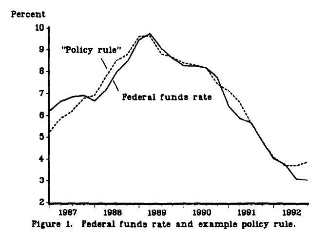
Source John B. Taylor, Discretion Versus Policy Rules in Practice, Carnegie-Rochester Conference Series on Public Policy, 1993.
Although it faithfully reproduces the Fed’s behavior over Taylor’s study period, this rule has since been criticized for various reasons, and has not always reproduced the behavior of central banks (see below).
Of course, it will come as no surprise to anyone that a rule as simple [as the Taylor rule] is unlikely to correspond to a fully optimal [monetary] policy.
Initial difficulties in determining the Taylor rate: calculating theoutput gap and the neutral rate
A first practical difficulty in determining the Taylor rate is estimating the various terms of the Taylor rule, notably theoutput gap and the “real neutral rate”, which are non-observable notions. The reference values of theoutput gap and the “real neutral rate” can be calculated in different ways, and the method of calculation can fundamentally change the results of the Taylor rule.
Output gap
As a reminder, the output gap is the difference between GDP and potential GDP. The difficulty in estimating theoutput gap lies in calculating potential GDP. There are numerous statistical and econometric models for estimating potential GDP. 24 Let’s take a look at two of them:
- One way of estimating potential GDP is to look at past data to estimate potential GDP at a given point in time (this is the principle of regression).25
- Another approach to estimating potential GDP is to start from the production forces (capital and labor) available at a given moment: from these values, and by estimating the country’s productivity, we can estimate potential production – and ultimately potential GDP.26
There is a whole range of methods for calculating theoutput gap. Depending on the method used and the assumptions made, the Taylor rate may vary – which limits the prescriptive nature of this rule. 27
Natural or neutral real interest rate
The natural rate (or neutral real interest rate) is a theoretical concept first defined by Swedish economist Knut Wicksell. 28 He defined the natural rate as the interest rate that balances savings and investment in an economy, without generating either inflation or deflation.
This notion is based on a simplified representation of the economy in which the neutral interest rate would, according to Wicksell, set equality between the supply of capital (from savings) and the demand for capital (to finance investment). It should be noted that Wicksell introduced and justified this notion within a very specific theoretical framework: a moneyless economy where banks are the sole intermediary between entrepreneurs and savers, and where companies finance themselves solely through debt (and not by raising capital, for example). These simplifications make Wicksell’s conclusions fragile when applied to the economy as it is (with bankers and money creation in particular).
This approach to the natural rate has been discussed in depth, notably by Keynes, for whom savings and investment are equal in accounting terms. Moreover, this definition of the natural rate as an equilibrium rate assumes that the economy automatically converges to equilibrium (on all markets) – something Keynes disputed.
Taylor’s rule, however, uses this concept. 29 In some versions of this rule – including Taylor’s original version – the natural rate is assumed to be equal to the economy’s “trend” (or potential) growth rate. However, this has no clear economic basis.
Central banks and international institutions use the natural rate as a reference rate (which would neither cause inflation nor deflation). However, this notion remains theoretical and unobservable, and can only be estimated via models and under strong assumptions.
The natural rate of interest cannot be directly observed, and its estimation is complex due to the challenges associated with measurement and model specification. In practice, estimates of the natural interest rate and their interpretation always depend on the model used and the data available, making them subject to both model and statistical uncertainties.
The choice of coefficients in the Taylor rule
As mentioned above, there is also the question of the coefficients applied to the gap between observed and target inflation, on the one hand, and to theoutput gap, on the other. In the 1993 versions by Taylor and Goldman Sachs (1996), these two coefficients were set at 0.5. These values were chosen empirically by Taylor as they provided a good representation of the evolution of Fed rates over his study period (1984-1992).
But there are other versions of the Taylor rule. 30 Here, we simply quote Taylor himself (1999) 31 who took up a work by Laurence Ball 32 and suggests applying a coefficient of 1 to theoutput gap. 33 In this way, the Taylor rate becomes more sensitive to a variation in theoutput gap than to a deviation of inflation from its target set by the central bank. It should be noted, however, that changing these coefficients does not change the fact that, in a so-called optimal situation, we fall back on the theoretical “golden rule” cited above.
The question of data access
Finally, for the Taylor rule to be used in practice by central banks to determine their key rates, they need to have access, in real time, to reliable estimates of several macroeconomic variables (inflation, GDP). This limits the operational character of the Taylor rule.
As Ben McCallum noted in 1993 34 For the calculation of the neutral rate at date t, Taylor uses data unknown to the central bank at that date, due to the time required to calculate them. The same applies to GDP and inflation calculations – which take several weeks to be calculated by the authorities.
The first estimates of macroeconomic variables published by monetary institutions are then often revised retrospectively. An analysis of US data from the 1980-90s showed that this can lead to deviations in the Taylor rate of the order of one percentage point. 35
Although statistical and econometric estimates have improved considerably since the 1980s-90s, there is still a delay in obtaining certain macroeconomic data. For example, the Bank of England published its first estimate of UK GDP for the first quarter of 2024 on May 10, 2024 – almost 40 days after the end of the first quarter. 36 In France, Insee published its figure at the end of April 2024. 37
Empirical evaluation of the Taylor rule – US and European cases
Despite the difficulties and limitations mentioned above, it is still possible to determine a Taylor rate – either a posteriori, or by estimating it in real time.
Application of the Taylor rule for the United States
The graph below compares the Fed’s rates with those given by two Taylor rules:
Evolution of the Fed and Taylor rates (1985-2024)
Reading: In the first quarter of 2020, the Fed rate was around 0.15%. The 1993 Taylor rule would have prescribed a rate of around -2%; the 1999 Taylor rule would have prescribed a rate of -7%.
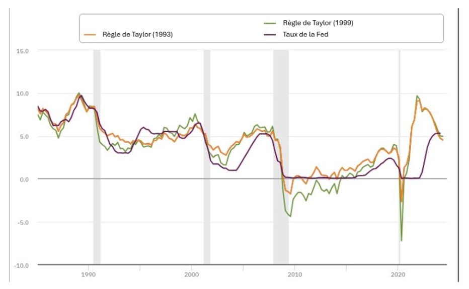
Source Taylor Rule Utility, Federal Reserve Bank of Atlanta.
Note: “Taylor’s rule (1993)” is Taylor’s original rule. “Taylor’s rule (1999)” is the other rule mentioned by Taylor in 1999, with a coefficient of 1 (not 0.5) in front of theoutput gap.
Different trends can be seen in the curves above.38
Between the 1980s and the early 2000s, the Taylor rule reproduces – with a few exceptions – the Fed’s key rates fairly closely. This period, often referred to as the “Great Moderation”, was marked by less volatility in the economic cycle – which, according to some central bankers, was due to the greater independence of central banks from politics, but which may be the result of many other factors (such as the relative stability of oil prices during this period). 39
From 2003 to 2005, Fed rates were below those recommended by the Taylor Rule, which Taylor believes contributed to the subprime crisis. 40 as the US economy was overheating.
During the 2009-2016 period, when the Taylor rule would have prescribed negative rates, the Fed kept its rates slightly positive, at around 0.15%, unlike some other central banks that implemented negative rates. 41 The same was true of the Covid crisis in 2020. In 2010, the Fed justified its decision not to cut rates below zero at such times by citing legal and operational constraints, as well as a lack of a clearly established framework – how far can it cut rates? 42
Finally, soon after the Covid pandemic, and in a context of galloping inflation, the Taylor rule would have prescribed a rate hike 1/ earlier, and 2/ larger than what the Fed did in 2022.
A word about negative key rates
In general, the key rates set by central banks are positive, meaning that commercial banks receive interest on the funds they deposit with their central bank. However, when a central bank sets a negative deposit interest rate 43 it forces commercial banks to pay to place their money with their central bank.
This phenomenon was mainly observed in Europe and Japan after the 2008 financial crisis, when central banks sought to stimulate the economy by encouraging spending and investment rather than savings. By encouraging banks to lend more, negative interest rates were intended to stimulate economic growth. The effectiveness of this measure was not really apparent, hence the use of quantitative easing .
Application of the Taylor rule for the euro zone
The graph below shows different Taylor rules (with neutral rates ranging from 0% to 2.5%) and compares them with the ECB’s main key rate, the MRO refinancing rate. 44 for the period 2014-2024.
The conclusions are similar to those for the United States:
- According to the Taylor rule, the ECB would have been too accommodating between 2017 and early 2020.
- At the time of the Covid crisis, in early 2020, the Taylor rule would have prescribed a far more significant cut in key rates than the ECB did. However, it should be noted that at the same time, the ECB launched a vast quantitative easing program (the Pandemic Emergency Puchase Programme, or PEPP). 45
- The Taylor rule would also have prescribed a rate hike 1) earlier, and 2) higher in the context of high inflation in early 2022.
ECB refinancing rate and different Taylor rates (for different neutral rates)
Reading: In Q1 2020, the ECB’s main refinancing rate was 0%, while the Taylor rule would have prescribed a key rate ranging from -5.5% to -8% – depending on the neutral rate used.
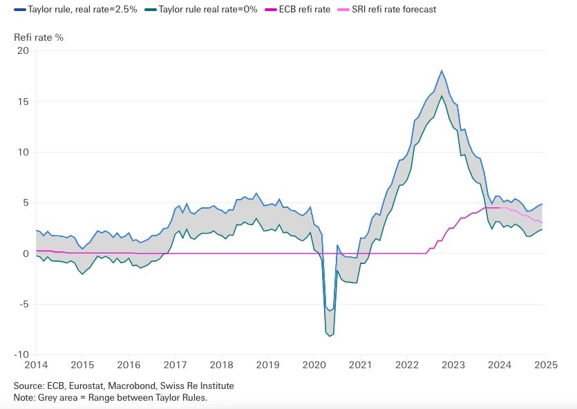
Source Charlotte Mueller, Diana Van der Watt, European economic outlook: wage growth holds the key to the interest rate cutting cycle, Swiss Re Institute (07/02/2024).
A few concluding remarks on the Taylor rule
Originally, the Taylor rule was not intended to be prescriptive, but rather to serve as a guide (among others) for the monetary policy stance of central banks. The rule uses a simplified, theoretical framework to simply link central bank policy rates – considered by international institutions to be the best way for a central bank to stabilize prices – to current inflation and GDP. Although frequently cited by international institutions themselves, it is inaccurate to say that the Taylor rule faithfully reproduces central bank monetary policy.
Empirically, the Taylor rule tends to react more strongly than central banks have to changes in economic conditions. Furthermore, during periods of low inflation, some central banks have developed other so-called “unconventional” tools, such as quantitative easing to stimulate the economy (which is not taken into account in the Taylor rule).
The yield curve
The Taylor rule thus imperfectly describes the evolution of central bank key rates. These rates are short-term rates (for periods of a few days or a week). This raises the question of potential links between short-term and long-term rates.
Theyield curve ( or term structure of interest rates) is the curve showing the interest rate (or yield) of a certain asset as a function of its maturity. 46
For example, in the case of government bonds – i.e. government debt – there are bonds with different maturities: 1-year bonds (after one year, the government must repay the amount invested plus interest) and 10-year bonds (repayment with interest takes place after 10 years).
Bond rates – i.e. the rates at which governments borrow – are very important variables, as they influence borrowing rates for individuals and businesses. 47 In the US, for example, real estate borrowing rates track 10-year government bond rates fairly closely.
Real estate rates follow government borrowing rates
Reading: In 1990, the US 10-year bond rate was around 9.2%, while 30-year mortgages had a rate of around 9.8%.

Source FRED Economic Data.
General case of the yield curve
In the general case, a yield curve has the following form:
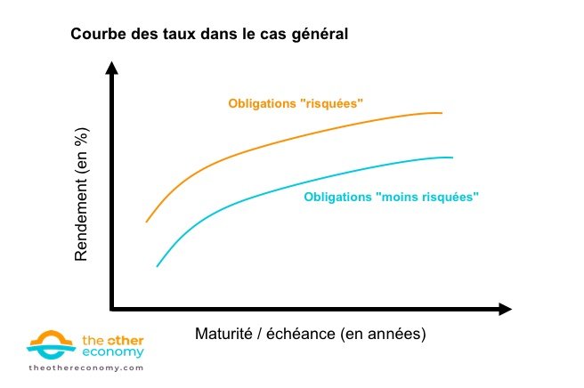
The longer the maturity of a security, the higher the (annual) interest rate, reflecting a risk differential: the longer the maturity, the greater the risk that the issuer of the security won’t be able to redeem its bond. There is therefore a “risk premium” or “term premium” when the maturity is longer.
Thus, the steeper the curve, the greater the risk premium investors demand for long-term lending.
Yield curve inversion
The above general shape of the yield curve does not always hold, however, and a situation known as inversion of the yield curve may arise. 48 Taking the case of bonds again, this occurs when short-term bond yields are higher than long-term bond yields.
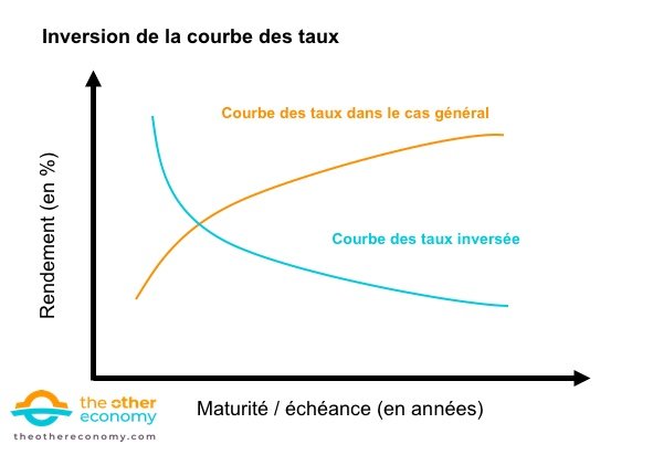
This is particularly true during periods of high inflation (such as 2022-2023 in Europe and the United States). 49 ). With inflation high, investors anticipate that the central bank will raise its key rates (short-term rates), which will tend to slow the economy (as the cost of financing rises). Short-term rates are therefore relatively high. However, investors also anticipate that medium- and long-term inflation will fall – and that the central bank will then lower its key rates. As a result of these expectations, medium- and long-term rates become relatively lower than short-term rates.
An inversion of the yield curve has historically been a harbinger of recession. However, the link between the two is still debated in economic circles. 50 Indeed, recessions (over the 1980-2020 period) in the USA and Europe have always been preceded by an inversion of the yield curve, but the reverse is not true. A counter-example is the European sovereign debt crisis (2010-2012), which was not preceded by an inversion of the yield curve.
Short- and long-term rates on the yield curve
Comparing long-term and short-term yields comes down to analyzing the shape of the yield curve. In the case of sovereign bonds, short-term bonds are generally defined as those with maturities of 1 or 2 years(1y or 2y ), while long-term bonds are those with maturities of 10, 20 or 30 years(10y, 20y and 30y respectively).
The evolution of short-term rates in relation to long-term rates is often observed through the spread, which corresponds to the difference (or gap) between these two rates over time. 51
The curve below illustrates the spread for US Treasury bonds. It represents the difference between the long-term US bond rate (10 years) and the short-term rate (2 years). A positive spread indicates a yield curve in its “general” case – i.e., the long-term rate is higher than the short-term rate. Conversely, a negative spread indicates an inversion of the yield curve, a phenomenon observed, for example, over the period 2022-2024, when the Fed significantly raised its key rate.
US bond spread illustrates yield curve inversion
Reading: In July 2019, the US 10-year borrowing rate exceeded the 2-year rate by 0.2 percentage points (corresponding to the spread).
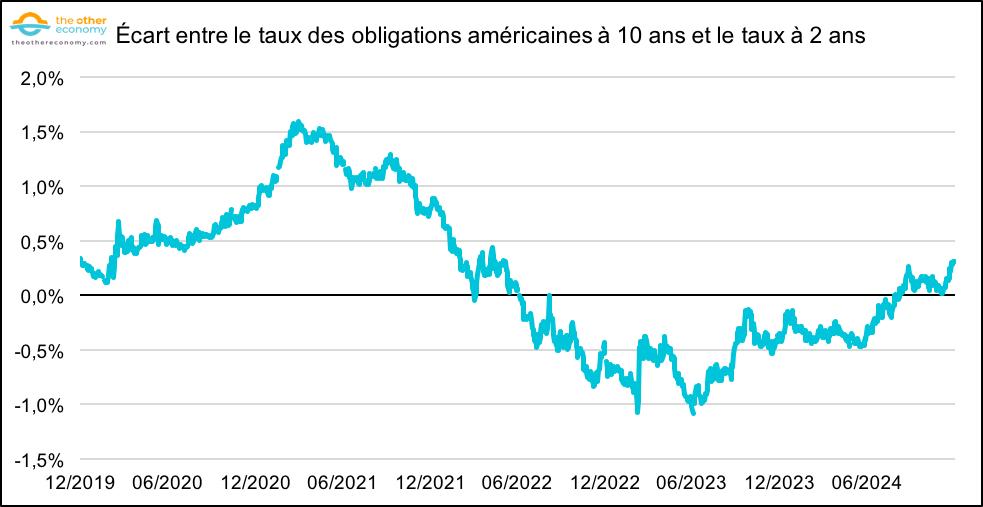
Source FRED Economic Data.
Dynamics and determination of long-term rates
The previous section presented some of the basic elements needed to understand the formation of the yield curve. Several economic theories have been developed in an attempt to explain it in greater detail, and to propose a rigorous model.
While there is consensus on the central role of central bank monetary policy in determining short-term rates, the determinants of long-term rates are the subject of much debate, with no clear conclusion.
The main classic models for long-term rates
Given the importance of long-term rates in the economy, various economic theories have been developed to understand their dynamics.
Anticipation theory
Expectation theory is the best-known approach – not least because it is relatively intuitive. This theory states that long-term interest rates reflect investors’ expectations of future short-term interest rates. 52 In other words, in its simplest formulation, this theory predicts that a long-term rate would be equal to the average of expectations of future short-term rates.
The underlying idea is that no one would invest in long-term bonds if investors anticipated that future short-term rates would be and remain higher than current long-term rates.
Indeed, if this were the case (present and future short-term rates higher than long-term rates), investors would prefer to invest in short-term bonds, and periodically reinvest in short-term bonds. Long-term rates must therefore correspond to investors’ expectations of future short-term rates.
Empirically, it is clear that investor expectations play a role in shaping the yield curve. However, the simplest formulation of expectations theory has been widely criticized, mainly because it neglects the risk premium associated with long-term rates. In addition, this theory is hampered by the inaccuracies of market forecasts of future short-term rates, calling into question its ability to fully explain the dynamics of the yield curve. 53
Forward guidance: an unconventional tool to guide financial players’ expectations
Since the early 2000s, several central banks have used a new, unconventional tool: forward guidance.
The principle is as follows: central banks communicate publicly on their future intentions in terms of monetary policy. In other words, they give indications of the likely direction of monetary policy in the medium and long term (raising, maintaining or cutting key rates, among others). 54
By communicating its future intentions, a central bank can guide the expectations of banks, investors, businesses and consumers – to the extent that it reduces their uncertainties about the future.
In so doing, central banks aspire, among other things, to influence long-term interest rates. For example, when policy rates and inflation are close to 0, the central bank’s ability to stimulate the economy through rate cuts becomes limited (as was the case in Europe and the USA in the 2010s). In this context, forward guidance becomes useful for signalling to the markets that rates will remain low for an extended period, which may encourage economic activity to pick up (and, in theory, drive inflation up).
Liquidity preference theory
The theory of liquidity preference is based on the idea that, without any particular incentive, investors prefer liquidity – i.e. the immediate availability of their assets – whether out of speculation or risk aversion. To encourage them to lend over the long term, it is therefore necessary to offer a risk premium – which generally results in long-term rates being higher than short-term rates, and thus justifies a fairly steep yield curve. 55
This approach explains why observed long-term rates tend to be higher than long-term rates predicted by expectations theory – the latter taking no risk premium into account.
However, taken in isolation, liquidity preference theory is sometimes considered simplistic, as it focuses on the supply and demand of liquidity, without fully integrating other important factors, such as monetary policy, default risks or market expectations. 56 By combining liquidity preference theory with expectations theory – which amounts to combining market expectations with a long-term risk premium – it becomes possible to analyze and estimate long-term rates more finely.
The chart below breaks down French and German 10-year bonds into two components: long-term interest rate expectations and the long-term risk premium.
Decomposition of French and German bond yields: market expectations and risk premium
Reading: In January 2020, the rate on 10-year French government bonds was around 0% (pink line), and this rate was even negative (-0.2%) for Germany (black line). The expected average of future short-term interest rates was 0.4% (grey zone), and the risk premium associated with securities issued from the Eurozone was -0.7% (red zone).
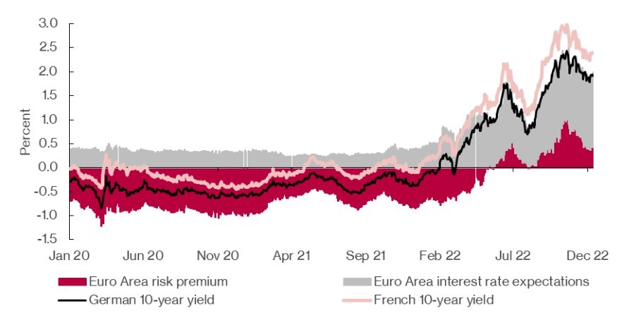
Source Paula Bejarano Carbo, Joanna Nowinska, NIESR Quarterly Term Premium Tracker, National Institute of Economic and Social Research, 2022.
Market segmentation theory
A third approach to understanding long-term rates is market segmentation theory. This is based on the idea that short- and long-term bond markets are more or less independent. 57 According to this theory, different investors prefer specific maturity segments according to their own financial needs. 58 For example, banks mainly buy and sell on short-term markets – because they need access to liquidity quickly – while pension funds participate more in long-term markets.
Interest rates for each maturity segment would thus be determined by the supply and demand specific to that segment – resulting in a segment-specific determination of interest rates.
In practice, studies show that certain short- and long-term rate trends can be amplified by market segmentation. 59 However, it would be insufficient to conclude that this is the only mechanism at play in the formation of long-term rates.
Other determinants of long-term rates?
The three best-known approaches to understanding the dynamics of long-term rates are presented above. That said, other characteristics of long-term rates have been studied in economic and financial literature.
A whole body of literature studies the potential “excess sensitivity” of long-term rates compared to short-term rates. Long-term rates would be particularly sensitive and could “over-react” to rapid variations in short-term rates. 60 More generally, this extreme sensitivity would reinforce the effects of monetary policy on long-term rates. 61 However, the amplifying effect of short-term rates on long-term rates is still under discussion in the economic literature. 62
The international context also plays a role in determining long-term rates (political stability, long-term rates in other major economies).63
Finally, we should mention unconventional central bank policies, in particular quantitative easing, which can have an impact on long-term rates – without central bank key rates changing. In effect, by buying up assets on the secondary markets 64 central banks are seeking to reassure investors and drive down long-term bond yields (since the price of the bonds in question will tend to rise). 65
EURIBOR and variable-rate loans
For long-term investments, companies and individuals can opt for variable-rate rather than fixed-rate loans, which means that the rate of their loan is revalued periodically (e.g. every year) according to market conditions.
To assess this variable rate, banks consult the value of EURIBOR, an interbank rate on the euro markets. 66 Every day, the European Banking Federation publishes various EURIBOR rates (for maturities ranging from 1 to 12 months). In concrete terms, these rates correspond to the average rates at which banks lent money to each other on the euro markets the previous day. 67 The variable rate is thus expressed as the sum of EURIBOR and the lender’s margin.
In fact, the 3-month EURIBOR – rated EUR3M – is one of the most closely scrutinized values on the markets. The UK equivalent of EURIBOR is LIBOR.
Long-term rates: financial products are determined by the markets
Ultimately, however, long-term rates are largely determined by the financial markets. Although models have been developed to better understand and predict long-term rates, this remains a difficult exercise. In recent decades, the yield on US 10-year bonds has almost invariably been overestimated. 68
Past forecasts have largely underestimated the decline in long-term interest rates. […] It is admittedly difficult to make predictions for the very long term, as many conditions can change over this horizon. However, even for shorter horizons, interest rate forecasts have often been inaccurate. Between 1984 and 2012, the U.S. Congressional Budget Office, private sector forecasters and the Administration all systematically overestimated the evolution of nominal interest rates, even just two years apart.
In addition to bonds, mortgages and corporate loans, there are many other financial products – such as derivatives – involving long-term rates (see box below).
An example of a long-term interest rate derivative: interest rate swaps (IRS)
A swap contract is an exchange contract between two parties. There are many such contracts. In the particular case of interest rates, there is the IRS(Interest Rate Swap).
The aim is to exchange interest on an initially fixed amount – known as the “notional amount”. In this operation, two parties, designated here as A and B, agree on the amount on which interest will be calculated. A undertakes to pay B a fixed interest rate – known as the “swap rate” – over a defined period. In return, B agrees to pay A a variable interest rate, the level of which depends on market conditions and the frequency of which is agreed in advance (every three or six months, for example). This mechanism makes it possible to exchange a long-term fixed rate for short-term variable rates.
In Europe, the variable rate is often based on EURIBOR, the rate at which banks lend money to each other (the American equivalent is LIBOR).
Based on all these observations, some researchers have pointed out that the price volatility of certain financial assets – in our case, long-term interest rates – does not necessarily reflect their intrinsic value, nor does it result from changes in other macroeconomic variables, but is the result of “extrinsic uncertainty” – i.e., with no direct link to the markets. Researchers David Cass and Karl Shell have introduced the metaphor of ” sunspots” to describe this phenomenon. 69
The complexity of long-term rate formation weighs on the ecological transition
The setting of long-term rates is complex and fluctuates according to market transactions – and therefore does not depend solely on the monetary policy of central banks.
Interest rates are a key tool for facilitating the ecological and energy transitions. By modulating the cost of capital, they can help or hinder the investments needed for these transitions. An adapted financial framework, with incentive rates for sustainable projects, is essential to accelerate the transition to a green and resilient economy.
- As explained in the note to the chart above, some central banks, such as the ECB, have several key rates. In the European case, two of these rates are lending rates. The last rate (deposit facility rate) is the rate at which banks can put their excess liquidity overnight. See : Les taux directeurs, ABC de l’économie, Banque de France, 2024. ↩︎
- Central banks also use other, unconventional tools, such as quantitative easing. See our sheet Understanding quantitative easing ↩︎
- See also criticisms by Keynes and Krugman: John Maynard Keynes, The General Theory of Employment, Interest and Money, 1936. Paul Krugman, The Limits of Purely Monetary Policies, The New York Times (16/12/2014). Paul Krugman, Money in a Time of Zero, The New York Times (03/09/2014). ↩︎
- See for example for France: Jean Pisany-Ferry, Selma Mahfouz, Les incidences économiques de l’action pour le climat, France Stratégie, 2023. ↩︎
- Simon Flowers, Peter Martin, How higher interest rates could hold up energy transition investment, World Economic Forum, 2024. ↩︎
- Emmanuel Macron, “Nous devons accélérer en même temps sur le plan de la transition écologique et de la lutte contre la pauvreté”, Le Monde (29/12/2023). ↩︎
- Principles for the Conduct of Monetary Policy, Federal Reserve, 2018. ↩︎
- See for example Politique monétaire, Réserve fédérale : Jay, John et les taux, Les Echos (14/12/2023) ; Le durcissement monétaire reste un sujet tabou, Les Echos (15/09/2022) ; The Fed policy error that should worry investors, Financial Times (26/01/2022). ↩︎
- This is the tool preferred by central banks, ahead of so-called non-conventional tools. ↩︎
- John B. Taylor, Discretion Versus Policy Rules in Practice, Carnegie-Rochester Conference Series on Public Policy, 1993. ↩︎
- Françoise Drumetz, Adrien Verdelhan, Taylor’s rule: presentation, application, limits, Banque de France. ↩︎
- John B. Taylor, Discretion Versus Policy Rules in Practice, Carnegie-Rochester Conference Series on Public Policy, n° 39, 1993. ↩︎
- Michael Woodford, The Taylor Rule and Optimal Monetary Policy, The American Economic Review, 2001. ↩︎
- The International Economic Analyst, Goldman Sachs, 1996. Quoted in: Françoise Drumetz, Adrien Verdelhan, Règle de Taylor : présentation, application, limites, Banque de France. ↩︎
- In the original version of the Taylor Rule, expected inflation is not included in the model – current inflation is. The addition of expected inflation was later proposed by Goldman Sachs. In particular, it makes it easier to deal with major, unforeseen shocks in the economy leading to a significant but temporary rise in prices (e.g. oil shock, see box above). ↩︎
- See our sheet Structural balance and potential GDP. ↩︎
- Typically, by not setting the two coefficients at 0.5 in the formula in front of p – p_target and in front of y – y*. In other words, monetary policy at a given point in time would depend not only on current macroeconomic variables, but also on past ones. ↩︎
- This is because the coefficient for both variables is 0.5. In other words, if theouput gap varies by 1, the Taylor rate varies by 0.5. ↩︎
- Sarwat Jahan, Ahmed Saber Mahmud, What Is the Output Gap?, International Monetary Fund, 2013. ↩︎
- Michael Woodford, The Taylor Rule and Optimal Monetary Policy, The American Economic Review, 2001. ↩︎
- For a review of the various classical and neoclassical models, see Jean-Marie Le Page, La hiérarchie du taux d’intérêt réel et du taux de croissance : une revue de la littérature et quelques constats empiriques récents, Économie appliquée, 2006. ↩︎
- Real interest rate = r_nominal – inflation = LT growth rate = r_neutral ↩︎
- For an empirical study up to 2004, see again: Jean-Marie Le Page, La hiérarchie du taux d’intérêt réel et du taux de croissance : une revue de la littérature et quelques constats empiriques récents, Économie appliquée, 2006. ↩︎
- Michael Woodford. Interest and Prices: Foundations of a Theory of Monetary Policy. Princeton University Press, 2003 ; Is the Output Gap a Faulty Gauge for Monetary Policy? | Richmond Fed; What Is the Output Gap? – Back to Basics – Finance & Development, September 2013 See also our sheet Structural balance and potential GDP. ↩︎
- Example: if average growth over the last 10 years is 2% per year, potential GDP for the following year will be 2% higher than observed GDP for the current year. ↩︎
- Karel Havik et. al, The Production Function Methodology for Calculating Potential Growth Rates & Output Gaps, European Commission, Economic Papers 535, 2014. In addition, other methods exist for calculating potential GDP, such as using business surveys to estimate excess supply or demand, which would allow us to estimate the gap between GDP and potential GDP. ↩︎
- Juan M. Sánchez, Output Gaps, Taylor Rule and the Stance of Monetary Policy, St. Louis Fed (04/03/2024). ↩︎
- Knut Wicksell, Interest and Prices, 1898. Note that the notions of neutral rate and natural rate are often interchanged. For a discussion of this topic, see: Josef Platzer, Robin Tietz, Jesper Lindé, Natural versus neutral rate of interest: Parsing disagreement about future short-term interest rates, VOX EU Columns, 2022. ↩︎
- Charles T. Carlstrom, Timothy F. Fuerst, The Natural Rate of Interest Rates in Taylor Rules, Federal Reserve Bank of Cleveland, 2016. ↩︎
- John B. Taylor, Monetary Policy Rules, University of Chicago Press, pp. 7, 1999. ↩︎
- John B. Taylor,A Historical Analysis of Monetary Policy Rules, 1999. In: John B. Taylor, Monetary Policy Rules, University of Chicago Press, 1999. ↩︎
- Laurence Ball, Efficient Rules for Monetary Policy, NBER Working Paper n° 5952, 1997. ↩︎
- Using the same notation as above, Taylor’s rule is: r_nominal = r_(real neutral) + p_anticipated + (y-y*) + 0.5 (p – p_target). ↩︎
- Ben McCallum, Discretion Versus Policy Rules in Practice: Two Critical Points. A Comment, Carnegie-Rochester Conference Series on Public Policy, 1993. ↩︎
- Athanasios Orphanides, Monetary Policy Rules Based on Real-Time Data, American Economic Review, 2001. ↩︎
- GDP first quarterly estimate, UK: January to March 2024, Bank of England (10/05/2024). ↩︎
- GDP grows moderately (+0.2%) in the first quarter of 2024, Insee (30/04/2024). ↩︎
- John B. Taylor, A Monetary Policy for the Future, Stanford University (15/04/2015). ↩︎
- See for example: The Great Moderation, Federal Reserve (22/11/2023). ↩︎
- John B. Taylor, Government as a Cause of the 2008 Financial Crisis: A Reassessment After 10 Years, Hoover Institution Economic Working Papers, 2018. ↩︎
- Janet L. Yellen, Comments on monetary policy at the effective lower bound, Brookings (14/09/2018); Mark John, Francesco Canepa, Era of negative interest rates unlikely to be revisited soon, Reuters (19/03/2024). ↩︎
- Ben S. Bernanke, What tools does the Fed have left? Part 1: Negative interest rates, Brookings (18/03/2016). ↩︎
- Negative interest rates, ABC de l’économie, Banque de France, 2022. ↩︎
- See also for a longer-term view: Economic Outlook Eurozone Q2 2024: Labor Costs Hinder Disinflation As Rate Cuts Loom and Assessment of the ECB’s current monetary policy stance. ↩︎
- ECB announces €750 billion Pandemic Emergency Purchase Programme (PEPP), European Central Bank (18/03/2020). ↩︎
- Maturity is the time between the date on which a bond is issued and the date on which its face value is redeemed. ↩︎
- For a bank, long-term bond rates (10, 20 or 30 years) correspond more or less to risk-free rates (assuming that the government will not default). To calculate the rate for a home loan to an individual, the bank takes this reference rate and adds a risk premium (depending on the borrower’s financial characteristics, etc.). ↩︎
- Matthieu Bussière, Stéphane Lhuissier, What does the inversion of a yield curve mean, Banque de France (25/01/2024). ↩︎
- Davide Barbusica, US Treasury key yield curve inversion becomes the longest on record, Reuters (21/03/2024). ↩︎
- Chelsea Bruce-Lockhart, Emma Lewis, Tommy Stubbington, An inverted yield curve: why investors are watching closely, Financial Times (06/04/2022). ↩︎
- This spread should not be confused with another well-known spread, the “OAT-Bund Spread”. The latter corresponds to the difference in interest rates between French (OAT) and German (Bund) government bonds of the same maturity (generally 10 years). ↩︎
- David O. Lucca, Samuel Hanson, Jonathan H. Wright, The Sensitivity of Long-Term Interest Rates: A Tale of Two Frequencies, Liberty Street Economics (04/03/2019); John C. Cox, Jonathan E. Ingersoll, Stephen A. Ross, A Theory of the Term Structure of Interest Rates, Econometrica,1985. ↩︎
- Massimo Guidolin, Daniel L. Thornton, Predictions of short-term rates and the expectations hypothesis of the term structure of interest rates, ECB Workshop on the analysis of the money market (working paper), 2008; Pasquale Della Corte, Lucio Sarno, Daniel L. Thornton, The expectation hypothesis of the term structure of very short-term rates: Statistical tests and economic value, Journal of Financial Economics, 2008; Warren J. Tease, The Expectations Theory of the Term Structure and Short-Term Interest Rates in Australia, Reserve bank of Australia, 1986. ↩︎
- James Lee, Sam Boocker, David Wessel, What is forward guidance?, Brookings (27/07/2023); What is forward guidance?, European Central Bank (15/12/2017); Christopher S. Sutherland, Forward Guidance and Expectation Formation: A Narrative Approach, BIS Working Papers, 2022. ↩︎
- Evelyne Jardin, Théorie générale de l’emploi, de l’intérêt et de la monnaie, Sciences Humaines (01/09/2003). ↩︎
- James Tobin, Liquidity Preference and Monetary Policy, The Review of Economics and Statistics, 1947. ↩︎
- John M. Culbertson, The Term Structure of Interest Rates, The Quarterly Journal of Economics, 1957. ↩︎
- Segmented Markets Theory, Corporate Finance Institute. ↩︎
- Aubhik Khan, The Role of Segmented Markets in Monetary Policy, Federal Reserve Bank Philadelphia, 2006. ↩︎
- Here’s one mechanism that may explain this “extreme sensitivity” of long-term rates to short-term rates (other mechanisms exist, but we won’t go into them here). Take the case ofyield-seeking investors. When short-term interest rates fall, these investors’ portfolios lose yield. As a result, they will tend to sell their short-term assets in favor of long-term ones – as we have seen with the yield curve in the general case, long-term yields are higher. These investors, having to change their asset portfolio, will accept a lower risk premium to keep overall returns high. See : Samuel G. Hanson, David O. Lucca, Jonathan H. Wright, Rate-Amplifying Demand and the Excess Sensitivity of Long-Term Rates, The Quarterly Journal of Economics, 2021. ↩︎
- Samuel G. Hanson, Jeremy C. Stein, Monetary Policy and Long-Term Real Rates, Journal of Financial Economics, 2012. ↩︎
- Dimitri Vayanos, Jean-Luc Vila, A Preferred-Habitat Model of the Term Structure of Interest Rates, Econometrica, 2021. ↩︎
- Christophe Blot, Jérôme Creel, Paul Hubert, Fabien Labondance, What factors explain the recent rise in long-term interest rates, OFCE (01/06/2017). ↩︎
- The primary market refers to the “new market”, where an issuer (government, company) introduces financial securities (shares, debt securities) for the first time. These securities can then be traded on the secondary market, also known as the “second-hand market”. ↩︎
- A bond pays a fixed rate of interest called a “coupon”. Let’s imagine a bond with a fixed coupon of €10 per year, purchased at €100 (i.e. a yield of 10%). If the market price of the bond rises, the bond’s yield – the ratio of coupon to bond price – falls. If, for example, the price of the bond rises from €100 to €110, with a fixed coupon of €10, the bond’s yield falls from 10% to 9.1%. So, the higher the price of a bond, the lower its yield. See : Quantitative easing, Bank of England (10/04/2024). See also our sheet Understanding quantitative easing. ↩︎
- What are reference rates?European Central Bank (11/07/2019). ↩︎
- Euribor, The European Money Markets Institute (EMMI). ↩︎
- Long-term interest rates: a survey, Executive Office of the President of the United States, 2015. ↩︎
- See : David Cass, Karl Shell, Do Sunspots Matter?,Journal of Political Economy, 1983. French researcher Nicolas Bouleau uses the term “smoke and mirrors markets” to describe markets where price fluctuations and investor behavior are primarily influenced by external factors or perceptions, rather than underlying economic fundamentals. See : Nicolas Bouleau, Les marchés fumigènes (05/12/2023). ↩︎