
This text has been translated by a machine and has not been reviewed by a human yet. Apologies for any errors or approximations – do not hesitate to send us a message if you spot some!
The central bank of a country (or zone) is an institution entrusted by the State with the task of implementing monetary policy. As explained in the module on money, the doctrine concerning the role of central banks and their means of action has evolved considerably over the course of history and from country to country. From the late 1970s onwards, in most advanced economies, attention focused on the objective of monetary stability, and in particular on controlling inflation, perceived as the major economic risk. Most central banks therefore adopted an inflation target of around 2%. The main monetary policy tool at the time was the key interest rate. Following the financial crisis of 2007-2008, Western central banks resorted to so-called “unconventional” policies, the main one being quantitative easing (QE). 1 . In this fact sheet, we’ll explain what quantitative easing is, which banks have implemented it, and what effects it has had on the economy, the ecological transition and inequalities. We will also address the thorny question of the consequences of exiting quantitative easing.
Changes in central bank monetary policies
Let’s start by reviewing a few points that are essential to understanding quantitative easing. For further details, please refer to the section on monetary policy in the Money module.
A country’s central bank is sometimes referred to as the “bank of banks”. Every economic agent (household, company) has an account with a banking institution. Similarly, every bank has an account with the central bank. This account is supplied with central bank money, the currency created by the central bank. However, central bank money can only be used for exchanges between banks – in other words, it does not circulate between other economic agents (households, businesses, non-bank financial institutions, etc.). In this context, the monetary policy pursued by central banks primarily consists of supplying central bank money to banks and setting its price.
The interest rate, the main tool of conventional monetary policy
When a bank needs a monetary base 2 it can either borrow it from another bank on the interbank market, or borrow it directly from the central bank. The central bank can also provide monetary base by purchasing debt securities held by banks. These two tools (loans and purchases of securities) have been used differently by the various major central banks: the European Central Bank favors the lending tool, while the American central bank (the Federal Reserve, known as the Fed) and the Bank of Japan make greater use of securities purchases (see section 3).
Central bank loans, also known as refinancing operations, are very short-term loans, maturing in 24 hours, one week or a few months. The central bank sets the interest rates on these loans: these are the key rates. 3 .
Before the crisis of 2007-2008, key rates were the main tool of monetary policy. They influence all other interest rates: interbank rates, bond market rates and lending rates. They therefore have an impact on economic activity by increasing (or reducing) the cost of credit granted by banks to economic agents (households and businesses), and therefore the ability of these players to consume or invest through borrowing. In theory, the rise or fall in economic activity in turn has an influence on inflation, the control of which is, as stated in the introduction, one of the main objectives (if not the main objective) of most central banks in advanced economies.
The use of unconventional monetary policies
In response to the financial crisis of 2007-2008, central banks made extensive use of the key interest rate. In the eurozone, for example, it fell steadily from 4.25% in July 2008 to zero in March 2016. It only became positive again in July 2022, following the rise in inflation (in December 2024, it stood at 2.9%, having peaked at 4.5% in September 2023. Source: BdF).
However, this tool proved insufficient. As soon as the subprime crisis broke out in mid-2007, the interbank market came under initial strain: banks had less confidence in each other’s financial strength, and were therefore less inclined to lend to each other. Interest rates on the interbank market rose to astronomical levels in October 2008, following the collapse of Lehman Brothers. The interbank market came to a standstill: loans between banks came to a halt.
Faced with the risk of the financial system collapsing, central banks implemented so-called “unconventional” monetary policies, essentially providing massive amounts of liquidity (base money) to banks to prevent them from going bankrupt. 4 .
It was in this context that an unconventional tool, quantitative easing, gradually began to be used by the central banks of advanced economies (from autumn 2008 by the US central bank, the Fed, then by the Bank of England and the Bank of Japan, and finally from 2015 by the ECB in response to the European sovereign debt crisis).
Initially envisaged as temporary, quantitative easing policies have in fact become a permanent fixture in the central banks’ toolbox, due to the persistent deterioration in the economic situation.
Chronology of quantitative easing policies
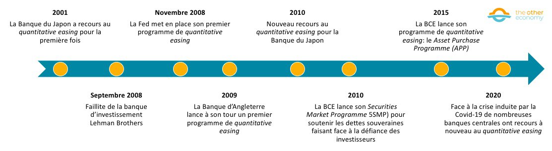
Source Le Quantitative easing, Banque de France fact sheet (2021)
Find out more
Educational publications from the Banque de France – ABC de l’Economie collection
What is quantitative easing?
Definition of quantitative easing
Quantitative easing consists of massive and prolonged intervention by a central bank in the financial markets, through the purchase of financial securities (mainly debt securities). 5 ), using the money it creates.
In most cases, the securities are bought from banks, but sometimes from other financial players as well. QE most often takes the form of asset purchases, i.e. operations carried out on the “secondary market” (see box).
Definition – Primary and secondary markets
The primary market refers to the “new market”, where an issuer (government, company) introduces financial securities (shares, debt securities) for the first time. These securities can then be traded on the secondary market, also known as the “second-hand market”.
While QE operations are mainly carried out on the secondary market, they can sometimes take place on the primary market: in this case, the central bank buys the debt security directly from the issuer. This practice is much less widespread, however, and is totally prohibited by European treaties for purchases of public debt securities.
Most QE programs have involved the purchase ofgovernment bonds. However, QE programs do not reduce government debt; they simply transfer ownership (since they are secondary market operations). This can be seen in many countries that have implemented quantitative easing policies, with the proportion of public debt held by the national central bank rising sharply between 2008 and 2022.
Share of national public debt held by the country’s central bank (in %).
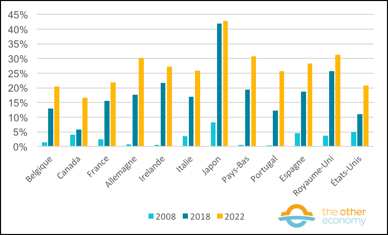
Source Database from the article Tracking Global Demand for Advanced Economy Sovereign Debt, IMF Economic Review, 2014. Although the article dates from 2014, the database (downloadable here) is regularly updated. Note: Values in Q4 2008 and 2018 and Q2 2022.
Reading: The Banque de France held 3% of French public debt in 2008, 16% in 2018 and 22% in 2022.
The stated objectives of quantitative easing policies
The quantitative easing can be mobilized to meet a number of central bank objectives.
Firstly, quantitative easing can be used to provide liquidity to banks when the interbank market is paralyzed, thereby preventing a collapse of the financial system. This is what the Fed did in November 2008, for example.
Secondly, QE is most often justified by the desire to deal with very low inflation, or even deflation, i.e. a prolonged fall in the general price level – since the price stability objective of central banks concerns not only inflation but also deflation.
As we saw in Part 1, in theory, when a central bank wishes to stimulate the economy, lowering its key rates enables banks to refinance at very low cost. This refinancing facility is supposed to encourage them to lend to households and businesses (by lowering long-term borrowing rates), thereby boosting the economy.
When key interest rates no longer work to stimulate the economy (i.e., when rates are already close to 0 or even zero), and inflation is close to 0, an economy is said to be in a ” liquidity trap “. As the outlook is poor, private players (households and businesses) are taking a wait-and-see attitude: even if interest rates are low, they are looking to reduce their debt or put money aside. They are also anticipating future price declines, and waiting before making purchases or investments.
In such a situation, central banks have to resort to other monetary policy tools, such as quantitative easing.
The massive purchase of securities (particularly government debt) by central banks is then supposed to have the following effects:
- Firstly, it increases banks’ reserves of central bank money, which should increase their ability to grant loans and thus boost economic activity: banks are less reluctant to lend, since they have easy access to central bank liquidity. In addition, QE reduces secondary banks’ holdings of government debt securities, thereby reducing their exposure to the risk of sovereign default. 6 .
- Secondly, QE increases demand for the securities bought back by central banks, driving up their price on financial markets. This automatically lowers the yield on securities already issued. 7 and, consequently, downward pressure on interest rates on new securities: access to debt is therefore cheaper for governments and companies that finance themselves on the markets. What’s more, as the yield on public debt securities acts as a benchmark for many other assets, including long-term lending rates to businesses and households, their fall will lead to a fall in borrowing rates for businesses and households (for property loans, for example), boosting the economy in theory.
- Finally, the fall in yields on debt securities will lead to a change in the behavior of banks and investors, who will switch from these assets to riskier, higher-yielding assets (such as corporate shares) or increase their lending to businesses and households, which is also expected to stimulate the economy.
All these mechanisms are thus expected to push up the general price level, thus removing the prospect of zero inflation.
Which central banks have used quantitative easing?
Quantitative easing in Japan
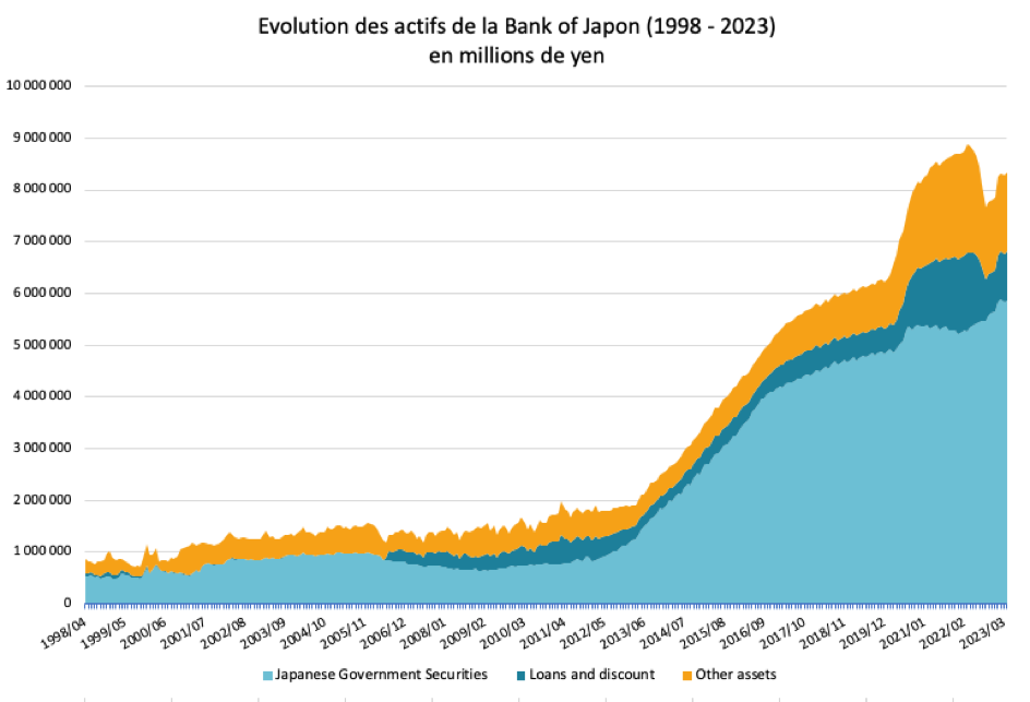
In March 2001, the Bank of Japan (BoJ) was the first central bank to adopt a policy of quantitative easing – two years after lowering its key rates to 0%.
During the 1980s, Japan’s overheated economy led to a bubble in asset prices (shares and land). The collapse of this bubble in the early 1990s profoundly disrupted the Japanese economy, culminating in the onset of recession in the late 1990s. 8 . To deal with this situation, the Bank of Japan was the first central bank to launch a QE program in 2001: between the beginning of 2001 and the end of 2005, the volume of government debt securities held by the BoJ almost doubled. This first program came to an end five years later, in March 2006, following the recovery of the Japanese economy. 9 .
In the wake of the financial crisis, the Bank of Japan announced a second program of asset purchases in 2010, and then, in 2013, accelerated its QE program, with a view to achieving its 2% inflation target within two years. The purchase of government debt securities was increased to 60-70 trillion yen per year (compared with 10-20 trillion yen in previous years). The peak will be reached in 2016, with 85 trillion yen of purchases, before gradually slowing down (but not stopping). In addition to quantitative easing, the Bank of Japan has been implementing other monetary instruments to stimulate the Japanese economy since 2012. All these economic policies are known as Abenomics, in reference to the Japanese Prime Minister of the time, Abe Shinzo.
In response to the Covid-19 crisis, the use of QE accelerates again in 2020. It is accompanied by other monetary measures, in particular loans to financial institutions (in return for the credit they extend to private players). For the first time since 2006, the Bank of Japan’s asset portfolio is temporarily reduced in 2022, as QE stagnates at the end of 2021 and the BoJ’s loan programs launched during the Covid-19 crisis come to an end: between March and September 2022, the value of outstanding loans granted by the BoJ as part of its Covid stimulus program is halved.
Quantitative easing in the United States
Open market operations( OMOs) are the Fed’s main monetary policy tool. They involve buying and selling securities on the market. Initially relatively limited in scope prior to the 2007-2008 crisis, the situation changed at the end of 2008 with the launch of four main quantitative easing operations. The change concerns not only the volume of securities purchased, but also their maturity (i.e. securities with longer maturities).
The Fed’s first QE program – often referred to as QE1 – was launched in November 2008, in the wake of the financial crisis. This program had a dual objective: to provide banks with liquidity – notably because they were no longer lending to each other – and to buy back mortgage loans. In total, through this program, the U.S. central bank bought $300 billion worth of U.S. Treasury bonds, $200 billion worth of public agency debt – companies “sponsored” by the U.S. Congress – and no less than $1,250 billion worth of mortgages.
The Fed’s second QE program, QE 2, began on November 3, 2010 and ended in June 2011, with the aim of stimulating the economy in a context of persistently high unemployment. This second program focused on buying back US Treasuries, for a total of $600 billion – and at a monthly rate of $75 billion in redemptions. Finally, the Fed added to this amount the income from the mortgages it held – bringing the total of this second program to $800 billion.
In September 2012, the Fed, observing an economic recovery that was too slow, launched a third QE program – in the hope of boosting business investment and lowering the unemployment rate 10 . Like QE1, QE3 involved both US Treasuries and mortgage-backed securities – for a total of $85 billion in redemptions per month. However, unlike previous programs, the US central bank did not specify either the duration of QE 3, or the total amount it would grant. In December 2013, against a backdrop of economic recovery and falling unemployment, it decided to reduce the monthly amount of repurchases and ended QE 3 in October 2014. 11 .
Finally, the Covid-19 crisis led the U.S. central bank to launch a fourth QE program, in March 2020 12 . With this program, the Fed increased its assets from $4.1 trillion in March 2020 to almost $9 trillion in March 2022.
Evolution of Fed assets (2002-2023) in billions of dollars
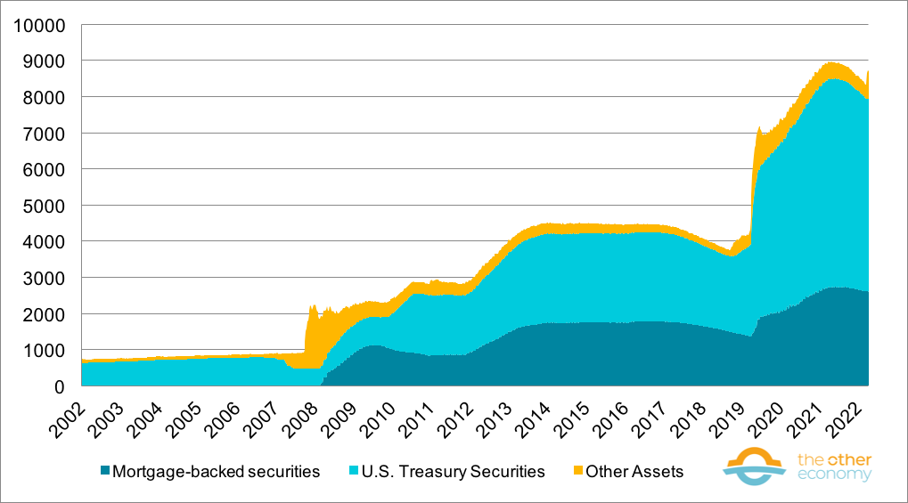
Source Fed balance sheet database (consulted on May 11, 2023)
The chart clearly shows the different phases of QE, with an increase in purchases of government debt securities and a massive surge in purchases ofmortgage-backed securities.
Since March 2022, the US central bank has progressively reduced its asset portfolio in order to bring inflation back to its target level of 2% – in a context where inflation was then at over 8%. As a result, its asset portfolio fell by just under 10% between March 2022 and March 2023 In March 2023, the collapse of Silicon Valley Bank (SVB) triggered a strong demand for liquidity from the US central bank by other banks: the Fed did not resort to a new QE program, preferring to support banks via loans (almost $300 billion was borrowed in one week 13 ).
Quantitative easing in the UK
The financial crisis of 2007-2008 was also the trigger for the Bank of England’s (BoE) first quantitative easing program. Although QE was initially envisaged by the Bank of England as a short-term measure in response to the financial crisis, it was subsequently used on several occasions. In total, five QE operations (known as Asset Purchase Facilities – APFs) were implemented in England between 2008 and the end of 2021.
The first three, between 2008 and 2012, were aimed at revitalizing the economy and providing liquidity to the banks. They involved a total of £375 billion of assets, or around 25% of UK GDP.
The second UK QE operation began in August 2016, following the Brexit vote announcing the UK’s exit from the European Union. As this decision agitated the financial markets, the Bank of England bought back £70 billion of assets on the markets – including £10 billion of corporate bonds – to encourage investors and banks not to abandon their slightly riskier assets in this very particular context 14 .
The third main QE operation, by far the largest, was launched in response to the Covid-19 crisis. Here, the Bank of England announced three rounds of asset purchases in March, June and November 2020, for a total of £450 billion of government bonds and a further £10 billion of non-financial corporate bonds – considerable amounts compared with the Bank of England’s first two major QE operations.
Since early 2022, following the example of other central banks, the Bank of England has begun to reduce its asset portfolio (by around 5% between early 2022 and early 2023).
Bank of England assets (2008-2020) in £ billions
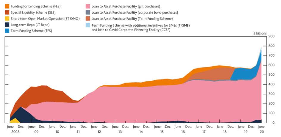
Source The central bank balance sheet as a policy tool: past, present and future – Bank of England (2020). Note: Loans to Asset Purchase Facility are the result of QE policies. They are mainly government debt securities (gilts).
Quantitative easing in the euro zone
The ECB (actually the Eurosystem, made up of the ECB and the 18 national central banks) launched its quantitative easing program much later than the other central banks. Indeed, the unconventional monetary policies implemented initially consisted essentially of providing banks with additional liquidity by granting them longer-term loans than those available under conventional monetary policy. 15 . The ECB refused to intervene in public debt, leaving the financial markets free to determine the cost. This is one of the reasons for the public debt crisis in the eurozone, during which interest rates in certain countries rose to such levels that they could no longer finance themselves on the markets. As this situation endangered the eurozone as a whole, the ECB eventually intervened.
In October 2014, the ECB announced the launch of a QE program: theAsset Purchase Programme (APP) for March 2015. Between then and December 2018, the ECB continuously bought back securities (from 15 to 80 billion euros per month). Between January and October 2019, it stopped buying new securities, while maintaining the overall amount of securities held. In other words, the ECB continued to reinvest the sums obtained by repaying the principal on maturing debt securities.
In total, the ECB’s asset purchases at the time amounted to almost €2,600 billion. Net repurchases resumed less than a year later, in November 2019. It was not until July 2022 that the ECB ended the APP (while maintaining the overall level of assets held). In February 2023, against the backdrop of a strong upturn in inflation, the Governing Council took the decision to start reducing the volume of assets held (by not fully reinvesting the principal of maturing debt securities).
Monthly net purchases by the European Central Bank under its Asset Purchase Programme (in billions of euros).
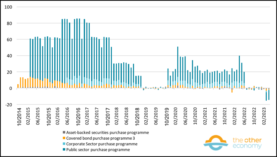
Source Asset purchase programmes – ECB website. Reading: in the first quarter of 2015, the ECB’s monthly net purchases under the APP were around €10 billion. They then rose to around €60 billion.
During the Covid-19 crisis, the ECB also launched the Pandemic Emergency Purchase Programme(PEPP) to support the public and private sectors, for a total of €1,850 billion.
Find out more
- History of QE policies for various countries – Bank of England document
- Explanations of the Fed’s open market operations and their evolution after 2008
- Details of the securities portfolio held by the Fed (System Open Market Account – SOMA)
- Quantitative easing: a dangerous addiction? Economic Affairs Committee UK Parliament (2021) – Chapter 1 Introduction – Quantitative easing and the UK
- ECB asset purchase programmes (APP)
- ECB’s Pandemic emergency purchase programme (PEPP)
How effective is EQ in practice?
First of all, unconventional monetary policies (including QE) prevented the financial system from collapsing in the wake of the 2007-2008 crisis, with all the devastating economic and social consequences that would have entailed.
In the longer term, while it is undeniable that QE policies have had an impact on the economy, it is difficult in practice to quantify their effects precisely, as Fed Chairman Ben S. Bernanke pointed out in his speech. Bernanke, Fed Chairman, in 2010: “To the extent that we cannot know how the economy would have evolved under other monetary policies, any answer to that question [that of the effectiveness of QE 1] is conjectural.” 16
The effects of quantitative easing on government bond financing
Despite these difficulties, the effects of QE on bond yields were evident. For example, in the two days following the announcement of the U.S. QE1 program, the yield on U.S. Treasuries fell by 107 basis points 17 . This case is also interesting insofar as it highlights the “signal” effect associated with a QE policy – capable of turning financial markets upside down even before the central bank buys back securities.
As explained above, this drop in yields leads to a reduction in the number of jobs. 18 medium- and long-term interest rates (particularly for government debt securities), thereby lowering the cost of debt for those affected by QE policies.
Yield curve for government bonds in the eurozone (AAA-rated)
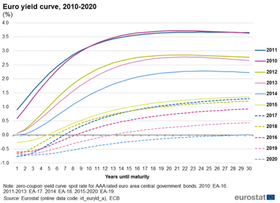
Source Eurostat – Statistics Explained: Exchange rates and interest rates – (see Eurostat database for exact statistics).
Reading: in 2020 (lowest blue dotted curve), AAA-rated government bonds with a remaining maturity of 1 year (i.e. due to be redeemed one year later) have a negative yield (around -0.6%); those with a remaining maturity of 30 years have a yield of less than 0.01%.
QE policies have therefore facilitated the financing of public debt, enabling governments to continue mobilizing their budgets to deal with the economic crisis following the 2008 financial crisis, and even more so with the consequences of the Covid-19 pandemic.
The effects of quantitative easing on economic activity
Despite the colossal amounts of monetary base created, the QE programs have not had the expected effects of large-scale economic stimulus – either in terms of growth in lending to households and businesses, or in terms of higher inflation.
As can be seen from the following graphs, after ten years of quantitative easing, the increase in liquidity injected into the banking system by central banks has neither translated into an increase in credit (and therefore money creation) in the same proportions, nor into an acceleration in inflation.
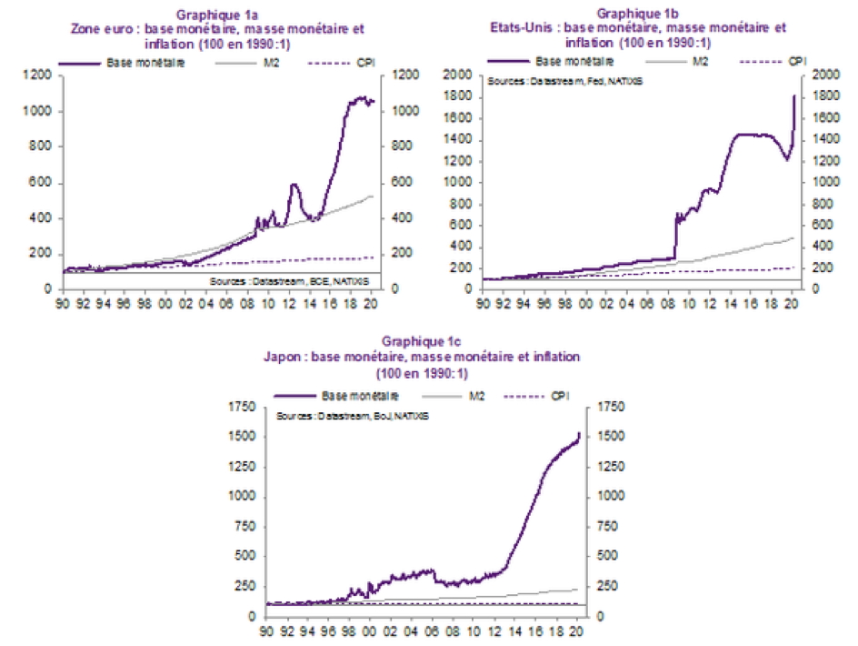
Source Natixis, Flash Economie, n°443, April 2020. Note: the increase in the monetary base reflects the creation of monetary base by central banks; the increase in the M2 money supply reflects the creation of money circulating in the economy by banks via their lending operations (see the Money module for explanations of the difference between the monetary base and the money supply, as well as the mechanisms of money creation by banks). The consumer price index (CPI) is the indicator used to measure inflation.
Indeed, banks cannot stimulate the economy in the absence of additional demand for credit from households and businesses. Although they are more inclined to grant credit when they have large reserves of monetary base, the trigger for credit is obviously demand. 19 from households and businesses. But demand depends on many factors, of which the availability of cheap credit is only one. The financial situation (income and debt levels) and confidence in the future (company order books, state of the labor market, etc.) also play a major role.
This observation highlights the inaccuracy of two widespread economic theories:
- The money multiplier theory (explained in the Money module), according to which any increase in the monetary base translates into a proportional increase in the money supply,
- The quantitative theory of money, according to which inflation is always the result of too much money being created (see our fact sheet on inflation and money). Despite ten years of quantitative easing, the level of inflation is correlated neither with the creation of central bank money, nor with money creation by banks.
However, the situation has changed since the end of 2021, with a return to inflation. This is no doubt partly due to the extremely massive QE put in place by central banks to deal with the economic consequences of the Covid-19 pandemic (notably by ensuring very low or even negative financing costs, so that governments are in a position to make up for the loss of household and business income caused by the shutdown). However, QE is far from being the only cause of the resurgence of inflation: tensions on product supply linked to the disorganization of supply chains due to repeated confinements (notably in China), tensions on the energy and food markets (resulting from the war in Ukraine), price-profit loops in certain sectors (where manufacturers are taking advantage of rising prices to increase their margins), etc. 20 .
The impact of quantitative easing on inequality
Another “mechanical” effect of the QE programs is to have maintained – and even encouraged and amplified – high asset values due to the increase in demand for these assets. This applies to securities that are the direct target of QE policies (government debt securities in particular), as well as to other financial securities and real estate assets, due to the abundance of available liquidity; the portfolio effect (financial players are looking for higher-yielding investments than government bonds); and low interest rates, which facilitate the use of debt and leverage. According to ECB studies, “monetary policy and the supply of mortgage loans have been the main drivers of the recent rise in house prices”. 21 .
This raises the question of the impact of QE policies on inequality. Indeed, the increase in the value of financial and real estate assets – a direct consequence of QE policies – enriches the holders of these assets: this is the wealth effect. This effect is highly unequal, since it enriches those who already have substantial wealth and are therefore among the wealthiest households. However, it should be noted that the effects of QE policies on wealth inequalities also depend on the nature of the assets purchased: the rise in real estate asset prices benefits more people – and in particular part of the middle class, who own their own home – while financial assets are almost exclusively held by the wealthiest households. 22 .
However, quantitative easing policies also have other effects, notably an income effect, which is more indirect than the wealth effect. The aim of QE policies is to revive the economy, which should ultimately benefit the entire population by reducing unemployment and – when inflation picks up again – raising wages. As periods of recession and high unemployment particularly affect the poorest households, this is a mechanism by which quantitative easing can help to limit income inequality.
In fact, various works 23 have been carried out to study the impact of QE on income and wealth inequalities. Ultimately, it is difficult to determine which of the two effects – the wealth effect or the income effect – prevails, and therefore to state whether quantitative easing contributes to an increase or a reduction in inequalities – all the more so as the wealth effect is an effect that may be short-term, while the income effect is a medium/long-term effect.
The impact of quantitative easing on the financing of the ecological transition
The neutrality of monetary policy is one of the main principles guiding the actions of central banks: they are not supposed to favor one economic sector over another, or one “economic policy” over another. While this principle is beginning to be challenged by the growing awareness, since the late 2010s, of the systemic risks posed by climate change to the financial system (see our module on finance), this has not yet translated into concrete action. For the most part, central bank policies to date have not been designed to encourage investment in the ecological transition.
It should be remembered that monetary policies have only an indirect impact on the financing of the economy.
QE policies do not directly provide additional liquidity to non-financial agents (companies, households, governments). When central banks purchase financial assets, they are generally pre-existing assets acquired on the secondary market. In so doing, they influence the price of the securities, but only indirectly on their supply, and very indirectly on the financing of the original issuers. Indeed, buying a debt security or a share at the time of issue does not have the same economic consequences as buying it on the secondary market: only the first option contributes directly to the investment by financing the issuer, while the second contributes above all to improving the liquidity of these assets and therefore lowering rates for bonds.
Moreover, while they facilitate credit conditions(by lowering medium- and long-term interest rates and facilitating access to central bank money for banking institutions), it is the banks that decide to whom to grant these loans. They constitute a permanent and inescapable filter between the actions of central banks and economic players.
The quantitative easing has tended to favor fossil fuel assets.
QE policies could have had an impact on the financing of the ecological transition. For example, it would have been possible to impose criteria on the assets eligible for QE, whether public debt or private securities (for example, by targeting green bonds or the shares of companies acting for the transition, or by excluding certain sectors such as fossil fuels). This is one of the proposals put forward by numerous experts and civil society organizations (see our User proposal for ECB quantitative easing to finance the ecological transition).
However, the application of the principle of monetary neutrality has prevented the implementation of such policies. In fact, the effect of QE has been quite the opposite: by being “neutral”, monetary policy has led to the perpetuation of the existing economic structure – which is largely based on fossil fuels.
For example, several studies have shown that the securities of private players acquired by the CBs as part of QE policies were largely from companies operating in sectors contrary to the transition. By way of example, under the ECB’s CSPP program – the private company debt repurchase program launched in 2016 24 63% of the securities bought back financed companies in sectors that emit the most greenhouse gases (fossil fuels, the automotive sector, power generation and “energy-intensive” industries). 25 . Another analysis even reveals that buybacks via the CSPP are clearly oriented towards sectors with high greenhouse gas emissions.
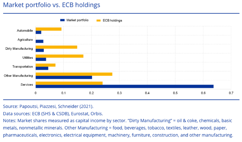
Source Speech by Isabelle Schnabel, member of the ECB Governing Council “From green neglect to green dominance? ” (March 3, 2021), citing the work of Papoutsi, Piazzesi, Schneider (2021).
The ECB was not alone. The same was true of the Bank of England’s CBSP private securities buyback program.
In response to this criticism, the two central banks have announced that they will gradually redirect their repurchases of private securities to limit their holdings of securities in sectors with high greenhouse gas emissions. 26 .
It should be noted, however, that private securities repurchase programs account for only a small proportion of the securities held by central banks, which mainly hold public debt securities. 27 .
Monetary policy tightening and quantitative tightening (QT)
For over ten years, banks and financial markets have been on a drip-feed of liquidity from central banks. As we shall see, getting out of this situation, and therefore putting an end to QE, is very difficult, and has numerous impacts on both financial stability and economic activity.
Tighter monetary policies
The rise in inflation from the end of 2021 has led to a tightening of monetary policy by most central banks – in application of the doctrine that central banks apply (and which is debatable, see our fact sheet on money and inflation). Initially, this took the form of a rise in key interest rates, which had repercussions on all interest rates in the economy. For example, the ECB raised its key rate for main refinancing operations from 0% to 3.75% between early summer 2020 and May 2023; similarly, the Fed’s key rate (the Federal Funds Rate) rose from 0.25% to 5.25% between March 2022 and May 2023.
In addition, several central banks have announced quantitative tightening (QT) programs, i.e. a reduction in the overall volume of securities held under QE (whether through the resale of securities or the non-reinvestment of volumes acquired when debt issuers repay principal). This is what the Bank of England and the Fed did as early as 2022, with decreases in asset volumes of the order of 5 to 10% over one year. The ECB, meanwhile, announced in early 2023 that it would also begin to reduce its asset base. Since January 1, 2025, the ECB has completely ceased all public asset purchases, whether under theAsset Purchase Program (maturing asset purchases ended in July 2023) or the Pandemic Emergency Purchase Program.
Monetary tightening and quantitative tightening: what are the risks for financial stability and economic activity?
After more than ten years of quantitative easing, and following the recent implementation of monetary tightening and quantitative tightening policies, it is also important to assess the risks that QE followed by a monetary tightening policy may represent for the economy from a financial stability point of view. While it is not yet possible to observe the full effects of such policies, we can attempt to identify them qualitatively.
For over a decade, very low interest rates have facilitated and encouraged certain economic players to take on debt, making them all the more sensitive to a tightening of monetary policy. This is obviously the case for governments, the primary targets of QE policies: higher interest rates lead to an increase in debt servicing costs as governments “roll over” their debt (i.e., re-borrow to repay maturing loans).
Above all, it puts the spotlight back on the unsustainability of public debt and the need to implement austerity policies by cutting public spending. As we explain in the module on public deficit and debt, policies advocating monetary tightening have harmful consequences for economic activity, as well as on social and ecological levels. 28 .
The priority given to fighting inflation by central banks thus comes at the expense of other economic policy priorities, such as the unemployment rate. As Jerome Powell, Chairman of the Fed’s Board of Governors, put it so bluntly in September 2022, the Fed’s program to bring inflation down to 2% (by raising rates and the QT) is likely to lead to higher unemployment. To justify this choice of monetary policy, the Fed pointed out that its primary objective is to maintain price stability – even if this means increasing the number of jobseekers.
The fallout from monetary tightening policies also affects other economic players.
Indeed, the rise in asset prices linked to quantitative easing policies has helped to sustain speculative bubbles, increasingly disconnecting financial markets from the productive economy. This was the case, for example, during the Covid-19 pandemic. The collapse of the world’s main stock market indices following the first wave of containment at the start of 2020 was short-lived: within a few months, prices had returned to or even exceeded their pre-crisis levels, while at the same time, the productive economy as measured by GDP was in recession. But this situation cannot last forever: every bubble eventually bursts. This is what we have seen in the tech sector . The difficulties of major digital companies, which were benefiting from a low-rate environment thanks in particular to the massive use of QE, were suddenly exacerbated by the implementation of monetary tightening policies and rate hikes, which ultimately had an impact on stock market prices. 29 . The case of smaller digital companies is also revealing. For years, digital start-ups were financed via debt and venture capital without the profitability of their business model being called into question. The downturn in monetary conditions, with rising interest rates, is causing difficulties in this sector, resulting in bankruptcies. 30 .
Finally, the downturn in monetary conditions is also having an impact on the banking and financial sector. There are two reasons for this.
On the one hand, as noted in the previous point, the bankruptcies of companies that lived by a permanent renewal of their debt and capital constitute losses for the financial players who lent them funds or invested in their capital.
On the other hand, rising interest rates and quantitative tightening policies cause the value of pre-existing financial assets to fall. Let’s take a concrete example: if you own a €100k ten-year government bond paying 0.1%, and the same government now issues ten-year bonds at 1%, the bond you own will lose value on the market (since nobody will want to buy it for €100k). This loss in value of existing securities is reflected in the balance sheets of the financial players who hold them.
In both cases, this poses a risk to the solvency of the financial players involved. These two reasons are among the main causes of the failure of Silicon Valley Bank (SVB), a regional bank specializing in financing digital start-ups, and of Credit Suisse, one of the world’s 30 systemic banks, which was bought out in an emergency in March 2023 by UBS (another systemic bank) with the help of the Swiss central bank.
Conclusion
Quantitative easing has become a very popular monetary policy tool since the financial crisis of 2007-2008. However, as we have seen, quantitative easing cannot replace fiscal stimulus in order to have a significant impact on the real economy, since it involves buying back assets on the secondary market. Moreover, quantitative easing would have greater legitimacy if it were directed towards assets that promote ecological transition (see the proposal for a QE geared towards ecological transition).
- As we shall see in the rest of this fact sheet, the Japanese central bank is an exception, having resorted to quantitative easing since the early 2000s. ↩︎
- Banks need central bank money for a variety of reasons, the most important of which is the need to settle what they owe to other banks as a result of transactions between their customers. For more on this subject, see the Money module. ↩︎
- Central banks generally use several key rates (the ECB, for example, uses three), depending on the duration of the loans granted. To find out more, see the Banque de France website and the educational fact sheet on key rates. ↩︎
- Without the central bank, a debtor bank would be unable to find the liquidity to pay what it owes, and would go bankrupt. As the players in the financial system are interconnected, this first failure, if it involves a “big” bank (known as systemic), would lead to a cascade of failures in other establishments. ↩︎
- To find out more, take a look at our module on public debt, where we explain how public debt securities are issued andhow they work. ↩︎
- Sovereign default occurs when a country is no longer able to repay what it owes to its creditors. ↩︎
- When the price of fixed-income assets rises, their yield necessarily falls: see the module on public debt for a numerical explanation. ↩︎
- Tamim A. Bayoumi, Charles Collyns, Post-Bubbles Blues: How Japan Responded to Asset Price Collapse. International Monetary Fund, 2000. ↩︎
- See the article, Il y a 20 ans, la Banque du Japon inventait l’argent gratuit, Les Echos (2019) and Effects of the Quantitative Easing Policy: A Survey of Empirical Analyses, Hiroshi Ugai, Bank of Japan, 2006. ↩︎
- See the Fed press release: Federal Reserve issues FOMC statement, September 13, 2012. ↩︎
- See Fed press releases: Federal Reserve issues FOMC statement, December 18, 2013; Federal Reserve issues FOMC statement, October 29, 2014. ↩︎
- See the Fed press release: Federal Reserve issues FOMC statement, March 15, 2020. ↩︎
- Michael S. Derby, Banks Sought record Fed liquidity in wake of SVB collapse. Reuters, March 16, 2023. ↩︎
- D. Milliken, A. Nicolaci da Costa, Bank of England wields stimulus ‘sledgehammer’ to beat Brexit blues. Reuters, August 4, 2016. ↩︎
- In the eurozone, these are first VLTROs (Very Long Term Refinancing Operations) and then TLROs (Long Term Refinancing Operations), which can have maturities of up to 3 years. ↩︎
- French translation by TheOtherEconomy. ↩︎
- A basis point is a hundredth of a percent, i.e. 0.01%. ↩︎
- See QE at the Bank of England: a perspective on its functioning and effectiveness – Quarterly Bulletin 2022 Q1 (Part 4). ↩︎
- See Alexander Rodnyansky, Olivier M. Darmouni (2017) The Effects of Quantitative Easing on Bank Lending Behavior, The Review of Financial Studies. ↩︎
- On these subjects see: ECB confronts a cold reality: companies are cashing in on inflation, Reuters, 2023 ; L’inquiétante flambée des prix des matières agricoles, Christian de Perthuis 2021 ; Ports bloqués, congestions de navires… le monde n’est encore pas sorti de la crise du covid-19, Novethic (2022) ; Faire face à l’inflation : un défi structurel, OFCE blog (2022) ; Looking through higher energy prices? Monetary policy and the green transition, Isabel Schnabel, ECB 2022; Exclusive: a profit-price loop feeds food inflation, C. Chavagneux. Alternatives Economiques, April 7, 2023. ↩︎
- Speech by Isabel Schnabel (ECB) Monetary policy and financial stability, 2021. ↩︎
- G. Clæys, Z. Darvas, A. Leandro, T.Walsh, The effects of ultra-loose monetary policies on inequality. Policy Contributions 885, Bruegel. ↩︎
- See for example: ECB Quantitative Easing (QE): What are the side effects? European Parliament, Monetary Dialogue June 2015; Quantitative Easing: What are the side effects on income and wealth distribution, DIW Berlin (2015). Quantitative easing: a dangerous addiction? Economic Affairs Committee UK Parliament (2021) – Chapter 2 Impact of quantitative easing – Distributional effects; M. Lenza, J.Slacalek, How does monetary policy affect income and wealth inequality? Evidence from quantitative easing on euro zone area. Working paper series 2190, European Central Bank; The distributional footprint of monetary policy, Annual Economic report, Bank of International Settlements, June 2021. See also Isabelle Schnabel’s speech at the ECB on November 9, 2021. ↩︎
- See amounts concerned in section 3.B. ↩︎
- S. Jourdan, W. Kalinowski, Aligning monetary policy with the European Union’s climate objectives, March 2019. Veblen Institute. For a detailed analysis of the CSPP as well as the Bank of England’s private asset buyback program, see: S. Matikainen, E. Campiglio, D. Zenghelis, The climate impact of quantitative easing. Granthman Research Institute on Climate Change and the Environment, London School of Economics, 2017. ↩︎
- For the Bank of England, see : D. Strauss, Bank of England to refocus corporate bonds on greener companies. Financial Times, November 5, 2021. For the ECB, see: M. Arnold, ECB set for greener ’tilt’ in €386bn corporate bond portfolio. Financial Times, July 4, 2022. ↩︎
- For example, in the UK, the CBPS envelope in 2021 was around £20 billion, representing less than 5% of the Bank of England’s securities portfolio (which, at its peak, was £895 billion). Similarly, the CSPP represents less than 10% of the ECB’s securities portfolio. ↩︎
- On this subject, see Isabel Schnabel’s speech (for the ECB) advocating monetary tightening in favor of the green transition – in particular to safeguard investment in renewable energy projects: Monetary policy tightening and the green transition, I. Schnabel, ECB, January 10, 2023. See also: Central banks should beware the dangers of over-tightening, P. Orszag. Financial Times, December 15, 2022. ↩︎
- On this subject, see the difficulties encountered by major tech companies in 2022, both in the real economy (resulting in massive layoffs) and on the financial markets (drop in financial valuation): J. Delépine, Pourquoi les entreprises de la tech licencient massivement? Alternatives Economiques, February 1, 2023; D. Tillaux, Gafam : l’année de la remise en question. Les Echos, January 10, 2023. ↩︎
- See on this subject: T. Kinder, Silicon Valley start-ups race for debt in funding crunch. Financial Times, December 19, 2022; E. Griffith, Silicon Valley Bank’s Collapse Chills Start-Up Funding. The New York Times, March 27, 2023. ↩︎