
This text has been translated by a machine and has not been reviewed by a human yet. Apologies for any errors or approximations – do not hesitate to send us a message if you spot some!
Derived from empirical observations, the Phillips curve, in its most elementary version, describes an inverse relationship between unemployment and inflation. Valid for many periods, it proved to be totally inaccurate in the 1970s with the onset of “stagflation”. It shows that statistical correlations can reveal important mechanisms, but do not exhaust explanations of the relationship between two complex variables. They are by no means “universal economic laws”. Furthermore, the debates surrounding the Phillips curve “myth” show how certain results can be instrumentalized to influence public policy.
What is the Phillips curve?
In 1958, the New Zealand economist Alban William Phillips (1914 -1975) published an article in which he demonstrated an inverse relationship between the rate of change in nominal wages and the unemployment rate in the UK over the period 1861-1957: the higher the unemployment rate, the lower the increase in wages. 1 . The reasoning behind this is clear: if unemployment is high, workers are prepared to accept lower-paid jobs for fear of unemployment. Conversely, in periods of low unemployment, they have a favorable balance of power to negotiate higher wages.
The Phillips curve in the Phillips article
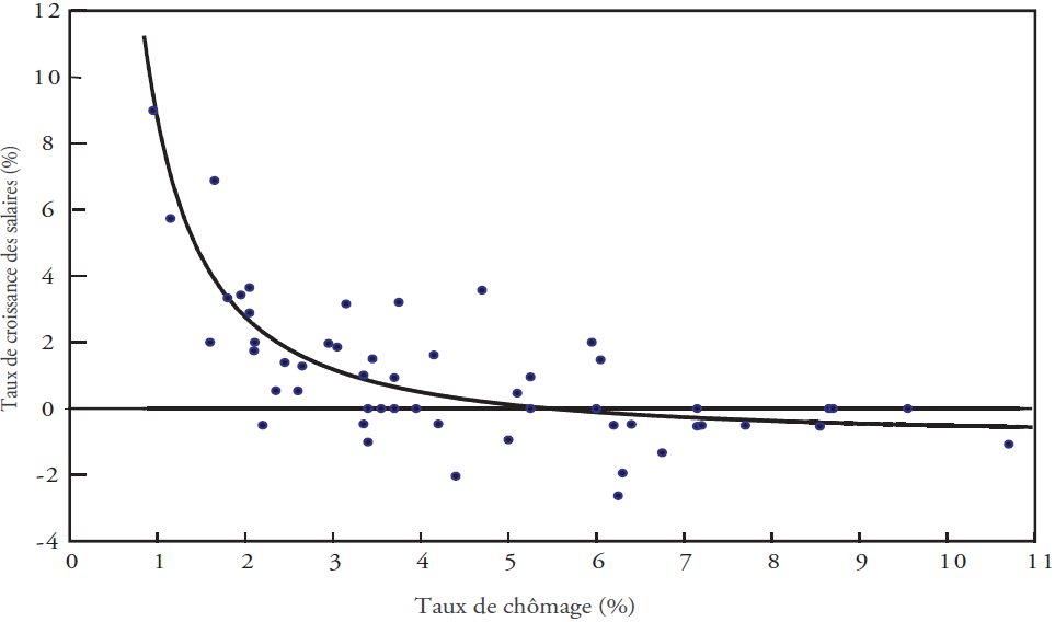
Source Alban W. Phillips, “The Relation between Unemployment and the Rate of Change of Money Wage Rates in the United Kingdom, 1861-1957”
This much-discussed curve is better known in a slightly different form: that of the link between unemployment and inflation. We owe this reinterpretation to
There are two reasons for this:
- Firstly, as labour costs are generally the most important production cost for companies, any increase in these costs can be passed on to sales prices;
- secondly, economists consider the unemployment rate to be an indicator (albeit an imperfect one) of the state of aggregate demand in the economy. The lower the unemployment rate, the more likely it is that the economy is in “good health”, and that demand for consumer and producer goods (investment) is relatively high. This high demand can create inflationary pressures if supply fails to keep pace.
The economists of the time never believed that this relationship represented an indestructible law of capitalist economies, and that such and such a rate of unemployment would correspond to such and such a rate of inflation for all eternity. They were well aware that, to put it graphically, the Phillips curve could move up or down.
The 1970s provided full-scale proof of this possibility, so much so that there was debate as to whether this curve actually “existed”. Indeed, in OECD countries, the 1970s were characterized on average by rising unemployment and inflation. This phenomenon was quickly dubbed “stagflation”, reflecting the almost unheard-of coexistence in developed countries of high inflation and periods of economic slowdown or stagnation.
The stagflation of the 1970s shows a more complex relationship between unemployment and inflation.
Beyond the debate over the existence of the Phillips curve (which reappears regularly), since the 1970s economists have highlighted several mechanisms influencing the relationship between unemployment and inflation, complicating the simple initial idea that low unemployment (or high aggregate demand) would push inflation upwards.
The role of inflation inertia and expectations
Because of negotiation habits and routines, but also because of the different types of indexation enshrined in law, if inflation is high in the preceding years, it is likely to remain high in the following years. 3 . As a result, an increase in inflation following an increase in aggregate demand (which supply cannot keep up with) or a supply shock (see point below) may be reflected in a permanently higher level of inflation in subsequent years. The expectations of economic agents also play a role in the evolution of inflation: if a majority of economic agents anticipate a rise in prices in the months ahead, this will be reflected in wage negotiations and between companies. 4 .
The existence of supply shocks
Commodity price shocks (such as the oil shocks of 1973 and 1979-1980) can have repercussions on prices in other sectors, temporarily raising the level of inflation. This additional inflation may persist due to inflation inertia and agents’ expectations. 5 . Such shocks can also reduce the overall productivity of factors of production, again leading to inflationary pressures.
The level of structural unemployment
In economics, we generally distinguish between cyclical unemployment, linked to cyclical fluctuations in the economy (greater or lesser activity), and structural unemployment, the consequence of changes in the structure of the economy, which may be due to demographic changes, the way the labor market functions, etc. 6 the composition and training of the working population, as well as job matching. 7 between workers’ skills and companies’ needs. In the USA in the 1960s, for example, the entry into the labor market of large numbers of women and African-Americans (who had previously remained outside the labor force) is said to have increased the structural unemployment rate. The result was higher unemployment, irrespective of the level of inflation.
How the “myth” of the Phillips curve has influenced public policy
Numerous macroeconomics textbooks written since the 1990s disseminate a history of the Phillips curve that economic historian James Forder has described as a “myth”. 8 .
According to the explanations given in these textbooks, governments’ belief in the Phillips curve led them to assume that they could arbitrate between low inflation and unemployment. It thus served as the basis for expansionary monetary and fiscal policies aimed at stimulating aggregate demand to reduce unemployment, in exchange for a few extra points of inflation. However, these demand-stimulating policies would have no effect on unemployment. Indeed, according to Milton Friedman, there is a natural (or equilibrium) rate of unemployment and, due to the gradual adjustment of economic agents’ expectations, it would not be possible, via demand-stimulation policies, to bring unemployment permanently below this equilibrium rate. 9 .
The popularity of the idea that there was a stable negative relationship between inflation and unemployment would therefore have been the source of the inflation of the 1970s, pushing up demand while having no lasting impact on the unemployment rate itself. This argument was devastating for Keynesian analysis at the time. Thanks to the “revolution” in economic thinking introduced by Friedman and the monetarists, policymakers would have understood that there was no long-term trade-off between inflation and unemployment, and would have rejected expansionary policies in favor of focusing monetary policy on price stability.
James Forder has clearly shown the inaccuracies and errors in this story. A thorough search of archives and administrative and political documents in the USA and the UK in the 1960s and early 1970s shows that the Phillips curve rarely came up in discussions, and that policymakers were far from believing that an all-out stimulation of demand could easily reduce unemployment in exchange for a few extra points of inflation. Moreover, Forder clearly shows that economists were aware, before Friedman’s arguments, that inflation inertia and expectations could play an important role, and that the Phillips curve was not a stable economic relationship.
However, since the 1980s, this myth surrounding the Phillips curve has helped to wrongly discredit the Keynesian economists of the 1970s, and with them expansionist policies. It also promotes an idyllic vision of the evolution of economic thought, which learned from its mistakes in the 1970s to arrive at a more adequate explanation of inflation thanks to Friedmanian analysis. 10 .
Finally, the myth of the Phillips curve wrongly tends to reduce the explanation of inflation in the 1970s to governments’ “blind” belief in the existence of a negative linear relationship between inflation and unemployment (leading them to pursue over-expansionary economic policies), and its disappearance in the early 1980s to monetary policies focusing on price stability, rather than unemployment. The reasons for this high inflation are, of course, much more complex and intertwined, as we attempted to outline in part 2. Today, most economists interested in this period tend to overlook the impact of rising oil and other commodity prices in the 1970s.
What do we think of the Phillips curve today?
If we look at the data for France (graph below), we can see the increases in inflation and unemployment at the end of the 1970s. From the 1980s onwards, the relationship between inflation and unemployment seems to follow the pattern described by Phillips, with rising unemployment accompanied by falling inflation (notably as a result of disinflation policies). The negative relationship between the two becomes weaker from the 1990s onwards: variations in unemployment over the period (which remains at a much higher level than in the 1970s) have no clear impact on inflation.
Nevertheless, the rise in unemployment in France following the 2008 financial crisis was accompanied by a slowdown in wage growth, and therefore a significant drop in inflation, tending towards 0, in line with the idea that there is a negative relationship between the two variables.
Inflation-unemployment pairing for France
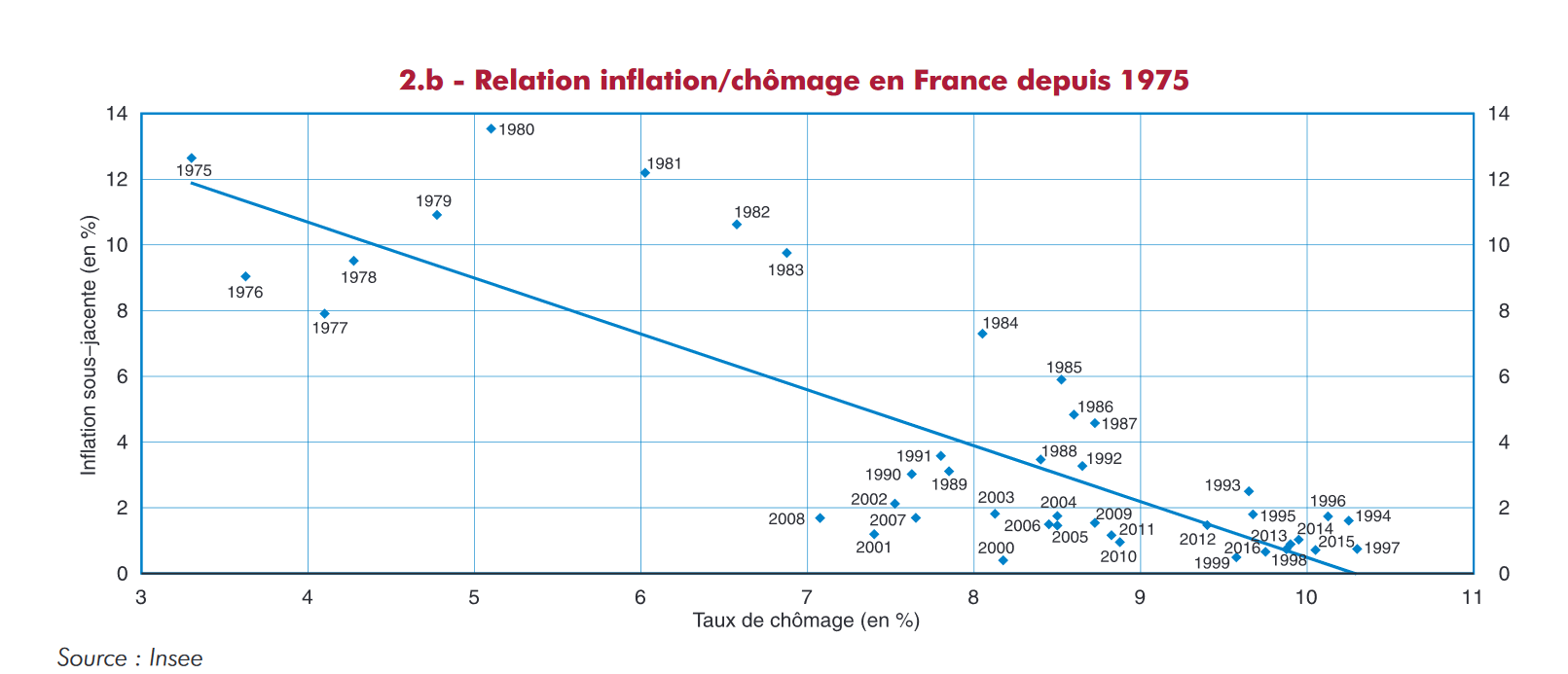
Source Benjamin Quévat, Benjamin Vignolles, “Les relations entre inflation, salaires et chômage n’ont pas disparu: étude comparée dans les économies française et américaine”, INSEE, Notes de conjoncture, March 2018.
Even if the negative relationship between inflation and unemployment, highlighted by Phillips in 1958, cannot be true at all times, in all places and at all times, it is nevertheless one of the pillars of our understanding of macroeconomic mechanisms.
Let’s add one last important point. The Phillips curve tends to focus attention on the measurement of inflation (calculated on the basis of the consumer price index, in France) and the unemployment rate. However, these are constructed data, produced according to a certain number of conventions, and as such they reflect more or less adequately, depending on time and place, the realities they are supposed to reflect. For example, unemployment is not always a good measure of underemployment (see the module on labor). We saw above that in the 1960s in the United States, it failed to account for the fact that women and African-Americans were, for the most part, excluded from the workforce.
Today, it does not reflect the very strong development of involuntary part-time work (i.e., people who would like to work more), nor the variations in the number of “discouraged unemployed” (who are not integrated into the working population because, through repeated failure, they have stopped actively looking for work) (find out more in the module on work). To better understand the relationship between inflation and unemployment, we therefore also need to look at differences in the underlying composition of unemployment, which is quite rare in Phillips curve analyses.
- Alban W. Phillips, “The Relation between Unemployment and the Rate of Change of Money Wage Rates in the United Kingdom, 1861-1957”, Economica, vol. 25, nᵒ 100, 1958, pp.283-99. ↩︎
- Richard G. Lipsey, “The Relation between Unemployment and the Rate of Change of Money Wage Rates in the United Kingdom, 1862-1957: A Further Analysis”, Economica, vol.27, nᵒ 105, 1960, pp. 1-31; Paul A. Samuelson and Robert M. Solow (1960), “Analytical Aspects of Anti-Inflation Policy”, American Economic Review 2, nᵒ 50, 1960, pp. 177-194. ↩︎
- Think, for example, of indexing the minimum wage to the previous year’s inflation. Similarly, it is conceivable that a sharp rise in prices could prompt trade unions to demand higher pay rises. The same applies to certain companies and their suppliers. ↩︎
- For a detailed and recent discussion of the Phillips curve and the role of inertia and expectations, see Olivier J. Blanchard, “The Phillips Curve: Back to the ’60s?”, American Economic Review, vol.106, nᵒ5, 2016, pp. 31-34. A presentation of the article, in French, was made by Martin Anota on his blog. ↩︎
- Robert J. Gordon, “The history of the Phillips curve: Consensus and bifurcation”, Economica, vol.78, n°309, 2011, pp. 10-50. ↩︎
- Some economists consider that the rules governing the labor market (minimum wage, dismissal procedures, etc.) constitute labor market rigidities that prevent wages from evolving in line with companies’ demand for labor, and thus lead to structural unemployment. ↩︎
- Matching problems occur when companies face certain labor needs that remain unsatisfied, because the skills required are rare in the workforce. There may also be geographical matching problems. For a summary of these mechanisms, see Sandra Pellet, Les mécanismes d’appariement sur le marché du travail, Regards croisés sur l’économie, vol. 13, nᵒ 1, 2013, pp. 25-30. ↩︎
- James Forder, Macroeconomics and the Phillips Curve Myth, Oxford: Oxford University Press, 2014. See also the following article summarizing this, Aurélien Goutsmedt, James Forder, Macroeconomics and the Phillips Curve Myth, Oeconomia 9-3, 2019. ↩︎
- The concept of the natural rate of unemployment is close to that of structural unemployment (even if Friedman’s main explanation was the “rigidities” of the labor market), with the difference that it is an “equilibrium” concept: the current rate of unemployment would always tend, in the long term, towards the natural rate. Consequently, the only way to reduce the unemployment rate in the long term would be to target the determinants of this natural rate (and thus, for Friedman, to make labor laws more flexible, reduce the minimum wage, cut welfare benefits,
etc. ). The principle of “hysteresis”, recently revived by Olivier Blanchard and Larry Summers, runs counter to Friedmanian logic: fiscal and monetary policies that reduce unemployment in the short term may enable employees to learn by doing, which would tend to reduce structural unemployment. See Olivier Blanchard, Lawrence Summers, “Rethinking stabilization policy: Back to the future”, Peterson Institute for International Economics, Conference paper, 2017. ↩︎ - Aurélien Goutsmedt, Les macroéconomistes et la stagflation: essais sur les transformations de la macroéconomie dans les années 1970, PhD thesis, Université Paris 1 Panthéon-Sorbonne, 2017. ↩︎