
This text has been translated by a machine and has not been reviewed by a human yet. Apologies for any errors or approximations – do not hesitate to send us a message if you spot some!
Since the Maastricht Treaty (1992), European Union member states have had to comply with two budgetary rules: the public deficit must not exceed 3% of GDP, and public debt must not exceed 60% of GDP. 1 . When a State exceeds these limits, an excessive deficit procedure may be initiated against it, leading to sanctions, including financial penalties.
The implementation of these rules, simple at first glance, has led to the adoption of two European Regulations (1997), amended and supplemented three times (2005, 2011 and 2013), followed by increasingly complex interpretative guides. 2 .
This corpus is better known as the Stability and Growth Pact. In 2020, the European Commission suspended the budgetary rules to enable countries to deal with the COVID-19 crisis. A new reform of the Pact is also envisaged.
The aim of this fact sheet is to present two non-observable indicators, “potential GDP” and “structural deficit”, which are now at the heart of European budgetary rules. We explain why they were adopted, how they are calculated, and their impact on member states’ budgetary policies.
Over the pages, we will discover that the difficulties encountered in recent years in bringing the reality of budgetary policies into line with the numerical rules of the Stability and Growth Pact are also the result of the accumulation of three flaws in the construction of these indicators:
- the methodological weakness of the underlying theories, which are unverifiable because they rely on unobservable variables,
- the difficulty of accurately measuring the variables associated with theoretical concepts,
- the probabilistic nature of the estimates, which should only be interpreted and used in the form of intervals and not single points. 3
Some of these developments will seem very complex. They reflect the technical nature of the rules themselves and the methods used to calculate the indicators; a technical nature inaccessible to the “layman” citizen, who doesn’t know what a “production function”, “total factor productivity”, or “unemployment that doesn’t accelerate inflation” is.
Yet, despite this technicality, the indicators used as a compass for budgetary policies cannot be validated according to basic scientific criteria. Behind these rules and calculations, presented as technical, lie political choices that limit the ability of governments to use the budgetary tool. Complexity thus becomes a formidable instrument for preventing public debate.
To find out more about the Stability and Growth Pact, budgetary rules and the various procedures that can be taken against States, consult our fact sheet on European economic governance;
You can also consult the module on public debt and deficit to understand the importance of budgetary policy and unravel the many misconceptions that surround the public debate on debt.
The Stability and Growth Pact: a restrictive interpretation of the Treaty
Balanced budgets: the cornerstone of the Stability and Growth Pact
The Treaty stipulates that before initiating an excessive deficit procedure against a Member State that fails to meet the 3% and 60% criteria, the Commission must draw up a report in which it takes account of the level of investment, the medium-term economic and budgetary situation, and “all other relevant factors”. The Council, acting on a proposal from the Commission and after an overall assessment, may or may not initiate the procedure. If the political will exists, this leaves a great deal of room for manoeuvre in terms of interpreting the excessive nature of the deficit. The Commission can also sound the alarm if a country is in danger of exceeding these reference values, and issue preventive recommendations.
The Stability and Growth Pact’s interpretation of the Treaty is based on the following principle:
compliance with the medium-term objective of a budgetary position close to balance or in surplus will enable member states to cope with normal cyclical fluctuations while keeping the public deficit within the reference value of 3% of gross domestic product
This interpretation, which is both prescriptive and incantatory, is highly restrictive: it places the pursuit of a balanced budget or even a budget surplus as the main condition for compliance with the 3% criterion.
The reason for this is that the budget balance, and hence the evolution of the public debt/GDP ratio, are not variables that can be precisely controlled by the public authorities (see box). The idea, therefore, is to aim for balance or surplus in good times, so as to have room for manoeuvre during economic crises, while respecting the 3% limit. This is the overriding principle, even if other relevant factors, such as exceptional circumstances beyond the government’s control, or a volume of investment meeting certain conditions, may be taken into account within strictly circumscribed limits (see point III.C).
Deficit levels, and hence public debt trends, depend on economic conditions
In a recession or economic slowdown, public revenues fall (e.g., lower consumption leads to lower VAT receipts), while expenditure rises due to the increase in social benefits, which are specifically designed to cushion cyclical shocks (e.g., rising cost of unemployment insurance, RSA, etc.). The deficit therefore rises mechanically if no new measures are taken; it falls just as mechanically when GDP growth picks up again.
Added to this is the impact on expenditure and income of exceptional and unforeseeable events, such as natural disasters, as well as the level of interest rates.
Source Find out more in the module on public debt and deficit.
How well have the criteria been met over the last few decades?
During periods of good economic health, member states have generally had no difficulty in complying with the 3% limit.
At the time, the vagueness of the Treaty and the wording of the 1997 Stability Pact enabled member states and the Commission to reach political agreement on the absence of excessive deficits or risks of such deficits, year after year. This was the case during the boom that accompanied the internet bubble at the turn of the 2000s, during the boom that preceded the financial crisis of 2007/2008, and during the timid recovery of 2016-2018.
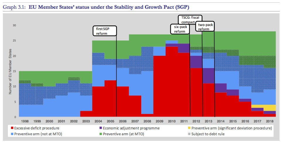
Source European Budget Committee: Assessment of EU fiscal rules, 2019 (p.27).
The red zones show the number of member states subject to an excessive deficit procedure. The blue, green and yellow areas show the number of countries whose deficits are not considered excessive, but which to varying degrees are considered at risk and subject to preventive measures. Cross-hatched areas show countries that are not respecting the rule of reducing their debt ratio towards the 60% limit.
But on two occasions, following the recession of 2004/05 and the Great Depression of 2009/10, the crises led to significant breaches of the limits set by the Treaty. This gave rise to disputes over the interpretation of these overshoots: were they solely the result of poor economic conditions, or were they also the consequence of pre-crisis budgetary decisions that were incompatible with the Treaty in the medium term?
To resolve conflicts of interpretation between countries, which are obviously political since national budgets are involved, the European Commission and the Council of Finance Ministers have been inclined to develop and include in the texts 4 increasingly sophisticated “techniques” designed to isolate the impact of the economic cycle on the budget balance from that of political decisions which affect the balance in the long term. This approach is intended to take account of the cyclical situation when assessing how quickly a country can reduce a deficit in excess of 3% or a debt level in excess of 60% of GDP. It also guides national budgetary policies in a preventive manner, even when the budget deficit remains below the 3% limit.
Potential GDP, its deviation from actual output and the structural balance, key variables in the Pact’s implementation mechanism
Potential GDP, a key but unobservable variable
The technique that has come to be used to isolate the budget balance linked to economic conditions from that due to political decisions is based on the assumption that production in an economy, measured by GDP, fluctuates around a potential. This “potential GDP” therefore represents the GDP that would be achieved when economic conditions are “normal”.
The difference between actual output (measured GDP) and “potential GDP” would then be used to determine the part of the budget balance due to the business cycle, while the other part, the so-called “structural” balance, could be controlled by the budgetary authorities.
In the publication by the European Commission’s Directorate-General for Economic and Financial Affairs (DG ECFIN) describing the calculations underlying the implementation of the Stability Pact, potential GDP is equated with “physical production capacity”. This is how it is described (P. 5).
“- In the short term, the physical production capacity of an economy can be considered as quasi-fixed, and its comparison with the evolution of effective/actual production (i.e. in the output gap analysis) shows by how much total demand can grow during this short period without causing supply constraints and inflationary pressures.”
“In the medium term, the expansion of domestic demand, when supported by a strong upturn in productive investment, can endogenously generate the production capacity needed to sustain itself. The latter is all the more likely to occur when profitability is high and supported by an adequate evolution of wages in relation to labor productivity.”
“- Finally, in the long term, the notion of full-employment potential output is more closely linked to the future evolution of technical progress (or total factor productivity – TFP) and to the probable growth rate of potential labor.”“”
The text continues:
“These medium- and long-term considerations should always be borne in mind when discussing potential output, as the latter is often viewed in an excessively static way in some policy-making forums, where capacity growth is often presented as invariant not only in the short term (when such an assumption is justified) but also in the medium and long term, as if the labor and total factor productivity (TFP) components of growth and their effects on fixed investment projections had no impact on productive capacity.”
In this definition, potential GDP thus appears as a fixed, “physical” and unobservable variable, but one that can leave traces through its interactions with other observable variables such as total demand, inflation, wages or investment.
Strictly speaking, since potential GDP is unobservable, estimating its level instantaneously according to the proposed definition presupposes not only an explanatory scheme for inflation and wages, but also the imposition of a norm on these two variables. We shall see in part III D that this is indeed the approach the European Commission is attempting to follow.
It should also be noted that in the medium term, potential GDP is likely to be influenced by economic policies and can therefore follow different trajectories. For example, a public policy favorable to investment (public and private) can increase production potential by enabling the development of new economic activities.
Potential GDP and structural balance, the compass for fiscal policy
We’ll see in Part III D that the method for estimating “physical productive capacity” (potential GDP) according to the definition proposed by DG ECFIN is based on questionable methodological and even political choices. These choices differ from one major international institution to another (IMF, OECD, DG ECFIN/European Commission). It is therefore important to understand how the estimation of this productive capacity determines the orientation of fiscal policies.
Intuitively, the idea is simple: the higher the estimate of potential GDP, and therefore the greater the gap between it and actual GDP, the greater the budgetary leeway available to the government to support demand (by boosting consumption or private investment, or launching public investments). It can therefore increase its spending by borrowing, without running the risk of running up against production constraints at a later date, which would prevent it from generating the net revenues needed to rebalance the budget without resorting to inflation.
Under the Stability and Growth Pact, a quantitative and operational measure of this budgetary margin is the so-called “structural balance”.
It is equal to the observed balance excluding interest paid on the debt, minus its cyclical component and minus exceptional expenditure due to events beyond the government’s control (natural disasters, industrial accidents, health crises, etc.).
The cyclical component is then deduced from the difference between observed GDP and “potential” GDP: this is known as the “output gap”. When observed GDP is lower than potential GDP, a cyclical deficit is created: tax revenues are lower than they would be in “normal” times, and spending, particularly social spending, is higher. Conversely, when observed GDP is higher than potential GDP, a cyclical surplus is created.
In other words, the structural balance excluding interest and exceptional expenditure is that which would have been recorded if GDP had been at its “normal” or “potential” level. When GDP fluctuates around potential GDP and the structural balance is constant, the cyclical surpluses generated during periods of high economic activity tend to offset cyclical deficits during periods of low economic activity. 5 .
This explains the importance attached to the structural balance as a compass for budgetary policies under the Pact. Properly controlled at a level “close to equilibrium”, it is supposed to make it possible to achieve the objective of keeping the (measured) current account deficit away from the 3% limit (barring exceptional situations such as the COVID19 health crisis). It would also make it possible to control the evolution of public debt on average over the economic cycle, since cyclical surpluses would tend to repay the loans taken out to cover cyclical deficits.
Choosing a method for estimating potential GDP means guiding budgetary policies
We have seen that budgetary rules oblige governments to make the structural deficit a fundamental criterion for the orientation of fiscal policy.
In concrete terms, the Stability and Growth Pact requires each member state to set a “medium-term objective” (MTO) for its structural balance, reviewed every three years. As we have seen, this MTO must provide a sufficient safety margin to ensure that the actual (measured) deficit does not exceed the threshold of 3% of GDP in a downturn. It must also allow for a gradual return to a level of debt below 60% of GDP, if necessary. 6 .
Alternatively, states must comply with an expenditure criterion. The gap between growth in potential GDP and growth in public spending (net of new tax receipts and certain social expenditure) must be compatible with achieving the medium-term objective for the public deficit. 7 .
The impact of a low estimate of potential GDP on public spending
The lower the estimate of potential GDP, the greater the constraint on net public spending, either directly or as a result of calculating the structural balance.
Indeed, if potential GDP is low, the difference with actual GDP will be slightly positive (or even negative if potential GDP is lower than actual GDP). As the cyclical component of the deficit is therefore relatively low, the estimated structural deficit will be relatively high (or, where applicable, the structural surplus low). In order to achieve their medium-term budgetary objectives, governments will therefore have to significantly reduce their structural deficits, and thus their expenditure net of new revenues.
According to one of the flexibility clauses in the Stability and Growth Pact 8 an alternative to cutting public spending is to carry out “structural reforms” designed to increase potential GDP (and thus reduce the calculated structural deficit) or public investment with a demonstrable effect on production potential. Reforms generally involve attempts to make the labor market more flexible, ease constraints (regulatory or fiscal) on the supply side (businesses) and encourage/facilitate innovation.
A low estimate of potential GDP may underestimate the risk of recession
Choosing a “conservative” estimate of production potential has its costs.
On the one hand, fiscal policy also has the function of attenuating cyclical fluctuations in economic activity by reducing taxes and/or increasing spending at the bottom of the cycle to support demand (or by increasing taxes and/or reducing spending at the top of the cycle to avoid overheating). As a result, an underestimation of production potential can lead to an overestimation of inflationary risks, as well as an underestimation of recession risks, and mask the need to support demand. On the other hand, it tends to constrain the ability to invest in public services and infrastructure.
To limit these risks, the effort required by the Pact to reduce the gap between the structural balance and the medium-term objective depends on the position in the cycle: it is all the lower the economy is in the low phase, i.e. when actual GDP deviates downwards from potential GDP.
In principle, therefore, the provisions of the Stability Pact make it possible to strike a balance between the two objectives, the legal one deriving from the interpretation of the Treaty, and the functional one making it possible to mitigate economic cycles.
But, as we have seen, the estimation of the structural deficit depends on the estimation of production potential. The balance to be struck between the different objectives therefore depends on the choice of method for estimating production potential.
It is understandable, then, that this apparently technical choice is a political issue, and had to be approved by the finance ministers. 9 .
Multiple sources of uncertainty and inaccuracy in estimating potential GDP and the structural balance
Inconsistent estimates that vary from one institution to another
Given the importance attached to potential GDP, the output gap and the structural balance in guiding fiscal policy, we would expect estimates of these variables to be at least robust, consistent and broadly consensual between the specialized institutions that produce them.
This is not the case, as shown in the table below. 10 .
Comparison of different estimates of France’s potential GDP and structural deficit
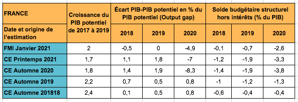
Source: AMECO Databank (Series 6.5 online and archive) and IMF, France’s Article 4 Consultation Report, January 2021.
- Regarding the level of potential GDP, there are significant differences between the assessment methods of the IMF and the European Commission (EC). For the IMF, France’s GDP was below or close to its potential in 2018 and 2019, whereas it was over 1% higher for the European Commission (EC). Furthermore, the estimate of the impact of the health crisis on potential GDP differs substantially between the Commission and the IMF.
- This results in significant differences in the estimated structural budget balance between the two institutions, even in non-crisis years.
- Retroactive revisions to the European Commission’s estimates of potential growth are substantial. For example, the output gap for 2018 was estimated at 0.1% of GDP in 2018 and 1.1% at the start of 2021.
Estimates increase the risk of counterproductive policies
Several analyses have also shown that estimates of potential GDP by various institutions, including those of the European Commission, are sensitive to actual GDP in the current period. As shown in the graph below, taken from an OECD study, a revision of the current GDP growth estimate by one percentage point was on average accompanied by a revision of the potential growth estimate by 0.18 percentage points.
A weakening economic situation therefore leads to a downward revision of production potential, and hence an upward revision of the structural deficit. Insofar as fiscal policy has a short-term impact on realized GDP growth, a retroactive loop can be created. To reduce the estimated structural deficit, the authorities pursue an increasingly restrictive fiscal policy. This has a negative impact on aggregate demand, and therefore on growth, leading to a further fall in the estimated production potential, and so on.
Sensitivity of potential GDP estimates to revisions in current GDP
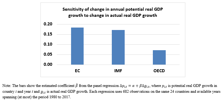
Source OECD Blog, If potential output estimates are too cyclical, then OECD estimates have an edge (2018)
In addition, for some authors, a cyclical weakening of GDP can have a real and definitive impact on potential GDP, according to a so-called hysteresis effect. 11 . Accelerated economic obsolescence of less profitable modes of production, loss of skills among unemployed workers 12 all these factors, which occur during an economic crisis, can have a lasting impact on production potential, even after the crisis has passed. The amplification of the fall in activity by a misguided fiscal policy then translates into a lasting fall in activity, accompanied by a lasting rise in unemployment.
It is therefore clear that it is not possible to steer fiscal policy solely on the basis of estimated potential GDP, without taking into account the risks identified above. This has been explicitly recognized by the European Commission, which has, for example, validated deviations of the structural balance from the required trajectory. 13 due to the “fragility of the recovery”, while the Pact’s flexibility clauses have become increasingly numerous and complex.
How the structural balance is calculated
The Commission calculates the structural balance in three stages.
> The first stage eliminates from the observed balance interest paid on public debt and expenditure incurred as a result of “exceptional” circumstances beyond the control of the authorities (natural disasters, industrial accidents, etc.). This conventional step leaves some room for political discretion. 14 but is not methodologically problematic.
> The second step determines the variation in the revenue and expenditure balance as a function of the variation in (measured) GDP. This is based on estimates of the relationship between tax revenues and GDP, and of the impact of GDP on spending, particularly social spending. Even if these estimates contain a degree of uncertainty, they are based on observable variables, and can therefore be assessed using verifiable statistical methods.
For example, according to the latest estimate 15 for France, one percentage point less growth mechanically increases the deficit by an average of 0.60 percentage points of GDP over a long period. However, this percentage may vary from one year to the next, depending on the state of the economy. Moreover, like all statistical estimates, it must be interpreted strictly as an interval within which the “true” value would lie with a certain probability, and not as a fixed point.
> The third stage is the least robust, yet the most decisive.
By estimating potential GDP, the cyclical component is set to zero, and only its variations as a function of changes in GDP are estimated at the previous stage. It is therefore at this stage that the level of the structural deficit, which will guide fiscal policy, is determined. Note that, for France, given the estimated impact of GDP on the cyclical component, a variation of 1% in the estimate of potential GDP upwards or downwards increases or reduces the estimated structural deficit by 0.60% of GDP, or around half of net public investment in 2019.
Calculating potential GDP: insurmountable methodological problems
As we shall show, the calculation of potential GDP multiplies assumptions that cannot be verified by observation, and sources of inaccuracy, whereas it represents an indicator that guides and commits to policies crucial to the harmonious and sustainable development of the European economy.
First method: extend past trends
One method sometimes considered for estimating potential GDP and its evolution is simply to extend the past trend in observed GDP, after eliminating cyclical fluctuations using conventional smoothing methods. The estimate of potential GDP then mechanically depends on observed GDP.
As mentioned in section 2.C, this dependence increases the risk of policies aggravating cyclical movements. This method also has the disadvantage of being conservative by construction, of not exploiting all available information, and of not providing a basis for reasoned projections.
Within the framework of the Stability and Growth Pact, a “theoretical” approach has been chosen.
It is based on a model that links GDP to observed variables, whose normal or potential level could be defined not only for the present, but also for the future. This model, described in detail in a European Commission methodological document 16 consists of two blocks.
> The first block assumes the existence of an identifiable and stable relationship between GDP and two aggregates supposed to represent, respectively, the stock of existing capital and the number of hours worked. In the long term, this relationship, represented by a “production function”, would evolve steadily thanks to “technical progress”, which would steadily increase the “total productivity of production factors”. This approach follows the growth theory proposed by Robert Solow. The production function is called Cobb-Douglas. In theory, this approach makes it possible to calculate the respective contributions of labor and capital to production and, by difference, to calculate the contribution of “technical progress”. Note that this so-called residual contribution is a calculated variable and is not observed.
> The second block assumes that, for the short term, it is possible to project the number of hours worked by making assumptions about the future rate of participation of the population in the workforce. 17 “rate, the “normal” unemployment rate and the “normal” or potential level of hours worked per job.
The participation rate and the level of hours worked per capita are projected by reference to past trends. The hypothesis used to identify the “normal” unemployment rate follows the Phillips curve hypothesis and its reinterpretation by the monetarist school. This theory defines the “normal” rate of unemployment as an “equilibrium” or “natural” rate at which there is no pressure to accelerate or decelerate wage trends. 18 .
To estimate the Phillips curve, and therefore the “normal” unemployment rate at time t 20 it is necessary to use an additional non-observable variable, “expected inflation”, statistically constructed from observed data. 19 .
As a result, estimates of potential GDP can only be interpreted as an interval and not as a single point. For the estimation of the structural budget balance, which depends directly on the level of potential GDP, this hazard is added to that resulting from the estimation of the mechanical impact of GDP on the budget balance.
The many methodological problems involved in estimating potential GDP render the method invalid
Over and above the probabilistic nature of potential GDP estimates, a few comments are in order to assess the relevance of the underlying theories and their ability to inform political decision-making. 21 :
- The assumption of the stability of a “physical” national production function over a long period of time is questionable in widely open economies, with increasing opportunities for companies to fragment, delocalize and relocate production chains and even services according to economic opportunities. Robert Solow himself pointed out the limits of his approach, notably that it should be reserved for “quiet trajectories with no stormy interludes”. 22 . This does not characterize the last twenty years, nor what we can expect from the upheavals in the production system that are essential to the energy transition. These uncertainties are also reflected in the existence of a “residual” variable that is nonetheless numerically significant 23 . Moreover, this variable remains unexplained by the model, but must nonetheless be projected to establish potential growth in the medium and long term.
- Similarly, the assumption of a working-age population that can easily be deduced from demographics is fragile in an economic area that guarantees the free movement of workers, either through temporary secondment or long-term migratory flows;
- The numerical translation of theoretical variables is itself a source of uncertainty and approximation. How can elements as disparate as public infrastructure, housing, offices, automobile production lines and blast furnaces be aggregated into a “single” capital stock, which would be a “physical” variable, when the only depreciation periods are the result of economic calculations? A similar problem arises when aggregating the hours worked by workers with different qualifications in very heterogeneous jobs. Is the relationship between hours actually worked and hours paid stable over the cycle? Do part-time or temporary workers work the total number of hours they want, or are they forced into unemployment, which is not reflected in the statistics? Does a falling participation rate really reflect a voluntary disengagement from the job search?
- The macroeconomic model used is partial and does not aim to take into account all the potential interactions between different macroeconomic variables. In particular, it is blind to possible interactions and synergies between fiscal and monetary policy. It simply pushes back to a limited number of other variables the need to identify the cyclical component and trend of the variables by smoothing the observations. As indicated in the Commission’s methodological note, this is the case for growth in “total factor productivity”, the labor force participation rate and the number of hours worked. The calculation of the so-called “natural” unemployment rate also fails to eliminate the cyclical component. 24 . The use of this macroeconomic model therefore offers only a marginal improvement over a method that simply calculates the trend in GDP from its observations. It also has the same shortcomings and risks.
The use of an unobservable variable renders the equation insoluble.
> On the one hand, even when estimates are based on theoretical assumptions linking the unobservable variable (potential GDP) to observable variables that can be projected in principle (hours worked, capital stock), the latter must necessarily be estimated using statistical methods that eliminate their cyclical component.
This ipso facto re-establishes the dependence of “estimated potential” on cyclical observations. This invalidates the assumption of short-term fixity of production potential and creates the risk mentioned in point 2.C of retroactive loops, or of overlooking important phenomena for guiding fiscal policies, such as the possibility of a lasting negative impact of a recession on production potential.
> On the other hand, to mitigate the cyclicality of estimates, it would be necessary to resort to increasingly complex theoretical models, taking the best possible account of retroactivity loops and the interactions of fiscal policy with other policies, in particular monetary policy, financial regulation and, where applicable, income policy. But “the” macroeconomic model that would decisively illuminate the future does not exist. There are only competing macroeconomic models, the validity of which has yet to be established, and which can at best be an aid to decision-making. 25 .
It is therefore understandable that the European Budget Committee and some observers suggest abandoning these complex calculations in favor of estimating potential GDP by simply projecting the trend. This would certainly increase transparency, but not relevance: for decisions involving medium- and long-term commitments, a simple extension of the trend is no guide. The right question, then, is the relevance of the underlying paradigm: should unobservable variables be used to guide fiscal policy?
In conclusion
The procedure for coordinating budgetary policies in the European Union is not currently based on a valid method.
For this to be the case, we need at least to be able to confront a theoretical hypothesis with observable, well-defined variables. The difficulties encountered in recent years in bringing the reality of budgetary policies into line with the numerical rules of the Stability Pact, resolved by multiplying the sources of flexibility, testify to the accumulation of three failings: firstly, the methodological weakness of the underlying theories, which are unverifiable because they make use of non-observable variables; secondly, the difficulty of accurately measuring the variables associated with the theoretical concepts; and thirdly, in any case, the probabilistic nature of the estimates, which can only be interpreted and used in the form of an interval and not a single point.
There is no need to abandon the intuition that a poorly implemented fiscal policy can lead to macroeconomic imbalances of various kinds, which will have to be corrected: inflationary pressures, too rapid a rise in the interest burden on debt, failure to meet climate targets, under-employment, insufficient investment in transition, increased inequality and insecurity… The reaction of economic production to additional public demand, whether or not financed by debt, is obviously an important factor to consider. To this end, the concept of “productive capacity” remains useful.
But we must radically abandon the idea that it is possible to determine and project a “production potential” and a structural balance that could be the supreme guide to public debt policy.
As DG ECFIN points out in the introduction to the methodological document already cited at the start of this note, the assumption of short-term fixity “of productive capacities” is not necessarily justified, and there are various possible medium/long-term trajectories for GDP. Each of these trajectories is associated, among other things, with different trends in employment, inflation, greenhouse gas emissions, inequality and public debt. Fiscal policy must be defined in relation to all these parameters, and not just in terms of debt and deficit.
- These provisions have been maintained in all subsequent treaties, and are now spelled out in Article 126 of the Treaty on the Functioning of the European Union and in Protocol 12 annexed to the Treaties. ↩︎
- See the list of documents on the European Commission website. This list is supplemented by publications from the European Commission’s DG ECFIN, the most important of which are mentioned in this note. ↩︎
- A campaign called “Output gap non sense” was waged by academics against the approach described in this note. It was based primarily on the lack of plausibility of the results and their economic and political consequences, rather than on criticism of the details of the method. See for example P. Heimberger ‘s note , “Output gap non sense – understanding the budget conflict between the EC and Italy’s government” (2019) with numerous references to this controversy. ↩︎
- This was achieved by revising the two main regulations of the Stability and Growth Pact (in 2005 and 2011), as well as in an intergovernmental treaty (the TSCG – Treaty on Stability, Coordination and Governance within the Economic and Monetary Union), which came into force in 2013. Read more in our note on the economic governance of the European Union. ↩︎
- In trend, because there is no guarantee of perfect symmetry between periods of overheating and economic slowdown. ↩︎
- The structural balance set as a medium-term objective should make it possible to reduce by one twentieth per year the gap between the debt ratio and the 60% norm. ↩︎
- See the Vade me cum on the implementation of the Stability Pact P. 27 ↩︎
- Find out more in our fact sheet on European economic governance. ↩︎
- For a review of position papers on this issue see European Parliament, Briefing, “Potential Output Estimates and their role in the EU fiscal policy surveillance” (2016). ↩︎
- …as well as in Appendix 2 of the European Parliament briefing , “Potential Output Estimates and their role in the EU fiscal policy surveillance”; See also the German note by Florian Schuster, Max Krahé, Philippa Sigl-Glöckner. ↩︎
- The concept of the hysteresis effect is borrowed from the physical sciences: it’s a phenomenon in which the effect persists even though its own cause has disappeared. ↩︎
- See O. Blanchard, “Should we reject the natural rate hypothesis?” Journal of Economic Perspectives (32,1), Winter 2018 ↩︎
- European Fiscal Board, 2019, “Assessment of EU fiscal rules”, P. 20 ↩︎
- These margins of appreciation concern, on the one hand, the level of expenditure considered to be “induced” and, on the other, the exceptional nature of the circumstances. ↩︎
- These estimates are updated regularly. See European Commission, DG ECFIN, Economic papers, No. 536, “Adjusting the budget balance for the business cycle: the EU methodology” (2014). Table 4.1, P. 21 for the estimate for France. ↩︎
- European Commission, DG ECFIN, 2014, Economic papers n°535, “The Production Function Methodology for Calculating Potential Growth Rates & Output Gaps”. ↩︎
- The labor force participation rate is a measure of the proportion of a country’s working-age population that is actively engaged in either working or seeking employment. ↩︎
- For a discussion of the Phillips curve and the “normal” or “natural” unemployment rate hypothesis see O. Blanchard, “Should we reject the natural rate hypothesis?”, Journal of Economic Perspectives (32,1), Winter 2018. The former IMF chief economist’s conclusion is that while the hypothesis of a non-inflationary unemployment rate may remain an attractive one, policymakers would be wise to have other options in mind. ↩︎
- For an exhaustive presentation of the methods used by the European Commission services, see European Commission, DG ECFIN, Economic papers n°535, “The Production Function Methodology for Calculating Potential Growth Rates & Output Gaps” (2014). ↩︎
- For a recent critique of the concept and its use to guide economic policy, see Jeremy B. Rudd, “Why Do We Think That Inflation Expectations Matter for Inflation? (And Should We?)” (2021). ↩︎
- An exhaustive discussion of the theories underlying these two blocks and their biases would go beyond the scope and needs of this sheet. ↩︎
- R. Solow, “The State of Macroeconomics”, Journal of economic perspectives (22-1), P. 244 ↩︎
- For France (P. 73), for example, potential growth in 2020 was estimated in 2019 at 1.25%, and is only half due to the sum of contributions from capital and labor. . The “residual factor”, calculated but not observed, therefore represents the other half of potential growth. ↩︎
- See European commission, DG ECFIN, Discussion paper 69-2017, “NAWRU Estimation using structural labor market indicators” (2017). ↩︎
- See A note comparing weather, climate and macroeconomic models co-authored by Gaël Giraud and Alain Grandjean; See also “The trouble with macroeconomics”, Paul Romer; “Do DGSE models have a future”, Olivier Blanchard, August 2018, Peterson Institute for International Economics. Policy Brief ↩︎