
This text has been translated by a machine and has not been reviewed by a human yet. Apologies for any errors or approximations – do not hesitate to send us a message if you spot some!
Launched in 1997, the Stability and Growth Pact (SGP) sets out in various legal texts the main principles of budgetary surveillance for EU member states, enshrined in European treaties since the Maastricht Treaty. In particular, this “Pact” aims to ensure compliance with two rules: the deficit must be below 3% of GDP, and public debt must not exceed 60% of GDP. The initial texts have been revised several times, with the latest reform dating from April 2024. 1 . They have also been supplemented by increasingly complex interpretative and methodological guides. However, the ideology underpinning the budgetary rules remains the same, and systematically leads us to seek to limit public spending – including investment.
The aim of this fact sheet is to explain, as simply as possible, how these rules are implemented in practice, the underlying economic reasoning, and to show their limits, particularly with regard to taking account of climatic drift. This simplification is a real challenge: the Commission’s notes on these subjects run to hundreds of pages. 2 and the whole thing is based on macroeconomic concepts that are difficult to understand and deeply debatable. The Commission has not produced a single summary explaining to the general public – or even to a well-informed public – the reasoning and logic behind this implementation; a summary which would nevertheless be necessary to enlighten national budgetary debates, which are heavily impacted by the SGP rules. This situation is certainly due to the fact that it is a construction made “between peers”. 3 who have received the same training, share the same beliefs and end up acting as if they were scientifically validated theories.
This fact sheet is therefore aimed at people who are already familiar with the workings of the EU budget and have a good basic knowledge of economics.
The purpose of budgetary rules
The philosophy of the Stability and Growth Pact, maintained in the 2024 reform, is as follows: an ideal situation would be one in which all countries pursued a fiscal policy that avoided, in all circumstances 4 a budget deficit in excess of 3% of GDP and to reduce and then maintain the debt-to-GDP ratio at a prudent level, below 60%. Consequently, based on a given budgetary situation, the regulations define the path that Member States must follow as a minimum to achieve this “ideal situation” over time.
The budgetary rules of the European treaties are not economically rational
There is no doubt that in an economic union, and a fortiori a monetary union, budgetary policies must be coordinated, and that such coordination can only be achieved on the basis of principles shared by all countries. It is also understandable that there should be a minimum requirement for debt sustainability .
The figures of 3% and 60% of GDP have, however, no serious economic justification. The 60% rate corresponds to the average public debt of the 12 countries of the European Union at the time of negotiation of the Maastricht Treaty; as for the 3% rate, as Guy Abeille, a witness at the time, explains, it was worked out on a corner of the table, one evening in June 1981, to meet President François Mitterrand’s conjunctural and political objectives.
And yet, these two “magic” figures are now considered criteria for debt sustainability, even though there are many examples of sustainable debt that do not meet them 6 including within the European Union. While the definition of debt sustainability may vary from one institution to another, there is a general consensus on the following terms: “Debt is sustainable when the borrower can be expected to continue servicing its debt without an unrealistically large correction in its income and expenditure”. 7 . A sustainability analysis is therefore always based on judgment, and cannot be reduced to the application of numerical rules.
There is no basis for such a general, quantified imperative common to all EU countries. These rules, set in the marble of the Treaties, are extremely restrictive and do not offer governments the flexibility they need to respond to the challenges they face.
More specifically, the Stability and Growth Pact has two components.8
The preventive aspect: organizing economic coordination between Member States, budgetary surveillance and preventing non-compliance with the rules
This is the purpose of the regulation on effective economic policy coordination and multilateral fiscal surveillance the legal basis of which is Article 121 of the Treaty (TFEU), which states that Member States shall regard their economic policies as a matter of common concern and shall coordinate them so as to contribute to the objectives of the Union.
Economic coordination has an austerity bias
Since the launch of the SGP in 1997, economic coordination, mainly centered on budgetary surveillance, has, by construction, led to a restrictive rather than expansive policy.
Firstly, budgetary trajectories are assessed according to essentially national criteria, and not in terms of overall EU dynamics. Secondly, the rules impose budgetary restrictions on certain States, but do not impose – or even encourage – expansionary policies on those States that could do so. This asymmetry carries with it the risk of seeing “austerity” policies for the whole of the European Union prevail on a regular basis.
Monitoring macroeconomic imbalances 9 introduced in the wake of the 2008-2011 crises, could have corrected this asymmetry and re-established an overview. However, this has not been the case, as this procedure has not acquired the weight of those relating to budgetary rules, and is also confined to a national approach. 10 Its reform was not envisaged at the time of the last reform of budgetary rules (completed in 2024).
The main stages of budgetary coordination resulting from the 2024 reform
Each Member State must submit to the Commission a national medium-term budgetary and structural plan covering the duration of a legislature (i.e. 4 to 5 years, depending on national circumstances).
The flagship indicator of these plans is the trajectory of net public spending 11 which must be consistent with European budgetary requirements (debt maintained or converging towards a level below 60% of GDP and a deficit below 3% of GDP over time).
Budgetary and structural plans also include explanations of the implementation of recommendations made by the Commission in previous years, as well as explanations of the reforms and investments carried out to contribute to the European Union’s priorities (in particular, equitable ecological and digital transition, social and economic resilience, energy security, and where appropriate, the strengthening of defense capabilities).
States that fail to meet the debt or deficit criteria are subject to a four-year period of budgetary adjustment. 12 They must then draw up (or revise) their medium-term strategic and budgetary plan, taking into account a “reference trajectory ” of net public expenditure transmitted by the European Commission.
Each budgetary and structural plan is assessed by the Commission and then validated by the Council, which formally adopts the net public spending trajectory that will serve as a reference throughout the adjustment period.
Trajectories can be recalculated at the time of each national election. They can also be recalculated if a country is placed under the excessive deficit procedure (based on the deficit criterion or the debt criterion), in order to “get it back on track”.
The corrective arm: the excessive deficit procedure
This is the purpose of article 126 of the Treaty and the Regulation aimed at speeding up and clarifying the implementation of the excessive deficit procedure .
According to the version of the Regulation revised in 2024, the following two criteria make it possible to declare an “excessive deficit”:
- the deficit criterion: the deficit is greater than 3% ;
- the debt criterion: debt exceeds 60% of GDP AND the budget balance is not in surplus or close to balance AND the country is not respecting its net public spending trajectory.
The deficit criterion is not automatic. Even if the budget deficit exceeds 3% of GDP, the Commission may not propose that the Council initiate a procedure, taking into account a number of well-defined relevant factors, such as the structure of the debt or the level of investment, including, according to the new regulation, investment in defense. However, it can only do so if the debt level is below 60% of GDP, or if the budget deficit remains close to 3%, and the projected overshoot is temporary.
Thus, in the first assessment under the new regulation (document dated June 19, 2024 ), the Commission proposed opening an excessive deficit procedure for only 7 countries, while 12 had budget deficits in excess of 3% in 2023 or 2024. (An eighth country, Romania, was already in excessive deficit).
To find out more about the various stages of the excessive deficit procedure, see our fact sheet on European Economic Governance (part 3.2.1)
The rationale behind European budgetary rules: the dynamics of the budget balance and public debt
Proposing a budget trajectory is no simple matter
The Commission, in liaison with national administrations, was tasked with making a static rule (deficit below 3% of GDP and debt below 60% of GDP) practicable and controllable in economies on the move.
It was therefore necessary to propose a method for defining, on a country-by-country basis, a trajectory for reducing deficit and debt-to-GDP ratios, year after year, for those countries that failed to comply with the rules.
In reality, this is a complex exercise. In fact, these two variables (deficit and debt) depend on numerous parameters that the authorities (national or European) have no control over, in particular: the interest rate on the debt, GDP growth in the short, medium and long term, which has an influence on public revenue and expenditure (as well as having an obvious influence on the ratio), cyclical fluctuations, the inflation rate, and so on.
The European Commission has therefore developed a specific method in conjunction with finance ministry officials, which we present below.
Identify the fiscal balance/GDP ratio that stabilizes the debt/GDP ratio
Let’s start with the simplest (relative to the rest) idea behind the definition of a budget trajectory.
Public deficit 13 is approximately equal to the increase in debt. Consequently, there is a level in the budget balance/GDP ratio that stabilizes the public debt/GDP ratio.
Let Y be GDP, d the primary public balance (i.e. excluding interest), r the interest rate, D public debt, g GDP growth in value terms (i.e. including inflation).
The total budget balance is equal to the primary balance, d, minus interest paid on debt , rD. It is therefore d-rD (budget equation).
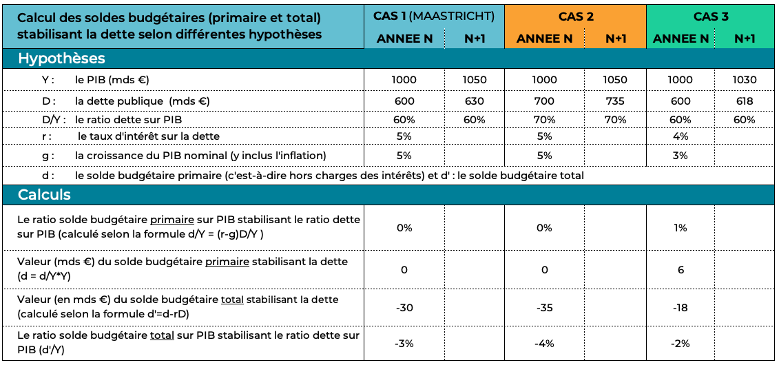
A few calculations show that the fiscal balance-to-GDP ratio(d/Y) “stabilizing” the debt-to-GDP ratio is equal to (r-g)D/Y.
Let’s take a few examples
If we take the values adopted at Maastricht (the famous 3% and 60%), with GDP growth in value terms of 5% (3% for real GDP and 2% for inflation) and a debt interest rate of 5%, the primary balance that stabilizes the debt must be equal to 0. The budget balance, including interest on the debt, is -3% (5% x 60%). These parameters stabilize the debt at its initial level, i.e. 60% of GDP.
However, this is not the case for the total budget balance (including interest), which depends on the level of debt. Given the same data for interest rates and GDP growth, if debt is 70% of GDP, then the total stabilizing budget balance is -3.5% of GDP (case 2 in the table below).
Finally, the situation becomes particularly difficult when the interest rate is higher than the growth rate (case 3 in the table below). For example, with a GDP of 1,000 billion, a growth rate of 3% and an interest rate of 4%, the primary balance as a % of GDP must be equal to or greater than 6 billion euros to stabilize the debt at 60%.
The hypothesis (cautious, or austere and unduly restricting investment, or arbitrary, depending on one’s point of view) adopted by the European Commission for the medium/long term corresponds to this case 3 . It requires all countries with debt levels close to or above 60% to achieve a positive primary surplus.
This reasoning has been considerably complicated by the Commission’s economists. 15 responsible for clarifying the rules to take account of a number of factors, which we will discuss in points 3, 4 and 5.
The return of public debt to a level below 60%.
As soon as public debt exceeds 60% of GDP, the debt ratio is not respected. To reduce this ratio, a lower primary deficit (or higher primary surplus) than the stabilizing balance is required.
The regulation resulting from the 2024 reform (preventive aspect), provides for a four-year adjustment period (or seven years if the country commits to an ambitious investment or reform program). On average, over this adjustment period, the debt-to-GDP ratio must “plausibly” fall by 1% of GDP per year if this ratio is above 90%, and by 0.5% of GDP if it is between 60% and 90%.
At the end of the adjustment period, the debt-to-GDP ratio must remain on a “plausible downward slope” or be kept below 60%.
Taking into account the economic cycle and/or the economic situation and returning and then maintaining the budget deficit at a level below 3%.
It’s quite intuitive to understand that a public deficit can be due to a downturn in the economy (which causes tax revenues to fall and social spending to rise, to put it simply) or, on the contrary, it can be “structural”, i.e. independent of the economy and the business cycle.
Following this logic, economists break down the budget balance into structural and cyclical components.
Definition and calculation of the structural balance
To calculate the structural and cyclical components of the budget balance, economists distinguish between actual GDP and an unobserved potential GDP, which would be GDP under “normal” business conditions, essentially reflecting the possible mobilization of productive forces outside the economic cycle.
In other words, potential GDP is the GDP (not observed in practice) that would result from “full employment” of production factors.
Three comments on potential GDP
– Determining potential GDP is very difficult. Different institutions take different approaches to this task, which leads to different results. In particular, it depends on the definitions adopted for unemployment and full employment, as well as on estimates of the reaction of wages to the unemployment rate, which vary according to the period under consideration. These variables are also eminently political in nature, as the next point shows.
– According to the method adopted by the Commission, potential GDP is not the maximum possible GDP, but the one in which wage increases do not accelerate inflation. 16 This economic policy choice is consistent with the debatable and unverified hypothesis of a stable wage bill/capital income distribution in the medium term. This choice is also reflected in the model used to calculate the evolution of GDP (with a Cobb-Douglas function à la Solow, see below).
– This potential GDP is likely to evolve if, for example, public policies make it possible to mobilize more production capacity (mainly labor).
We detail the calculation of potential GDP, the choices on which they are based, and their limitations in our data sheet. Potential GDP and structural balance
The structural balance (i.e. excluding interest expenditure) is calculated from the difference between actual GDP and potential GDP, known as the output gap.
If the economy is under-performing (actual GDP below potential GDP), a cyclical deficit is created: tax revenues are lower than they would be in “normal” times, and spending, particularly social spending, is higher. Conversely, when observed GDP is higher than potential GDP, a cyclical surplus is created. The structural balance is the difference between the observed balance and this cyclical balance. It is important to note that this cyclical balance is obviously based on assumptions and not on observable data.
More precisely, the primary structural balance calculated by the Commission is equal to the observed balance excluding interest paid on the debt, the cyclical component, exceptional expenditure due to events beyond the government’s control (natural disasters, industrial accidents, health crises, etc.), and any other exceptional items. 17 ) and EU-funded expenditure. The structural balance is the primary structural balance, including expenditure on interest payments on the debt.
Structural balances in France, Germany and the euro zone over the 2000-2023 period
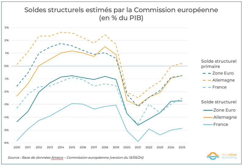
Source European Commission AMECO database (version of 15/05/24) – Series 17.1 (Structural balance and Structural balance excluding interest, % pf GDP)
The structural balance: a key indicator for budgetary surveillance
Structural balances (with or without interest expenditure) are key indicators used in budgetary surveillance. They are calculated in such a way as to ensure that countries “in good standing” continue to respect the debt and deficit criteria, and that the others respect them at the end of the 4 or 7-year adjustment period.
In concrete terms, the evolution of structural balances over the adjustment period is calculated to meet the following objectives.
- Firstly, at the end of the adjustment period, the structural deficit (including interest expenditure) must be less than 1.5% of GDP, to avoid a situation in which, even in the event of the “usual” cyclical downturn, the structural deficit would remain below 1.5% of GDP. 18 the real budget deficit does not exceed 3%. For a country declared to be in excessive deficit 19 the minimum adjustment of the structural balance is 0.5% of GDP per year. Until 2027, however, this condition only applies to the primary structural balance (i.e., the structural balance excluding interest payments), which will somewhat attenuate the adjustment at the start of the period for countries whose interest burden is rising.
- Secondly, the primary structural balance (excluding interest expenditure) must meet the conditions required to reduce the debt-to-GDP ratio or stabilize it at below 60% (see sections 2.2 and 3).
- It is then assumed that, at the end of the adjustment period, the primary structural balance will remain constant at a level which, barring exceptional circumstances, will enable the debt and budget balance conditions to be met over the following ten years.
The resulting adjustment to the budget balance is then translated into an accounting relationship 20 into a trajectory for net public spending, set at the beginning of the adjustment period. This last variable, which lies at the heart of the budgetary and structural plans that the Member States submit to the Commission, is the only one that will be “monitored” during the adjustment period to assess compliance with the regulations.
The changing terms of the budgetary equation
Controlling public debt and the overall budget balance (structural, cyclical and interest expenditure components) is a long-term process. To ensure this, we need to make projections for the key variables in our reasoning, and in particular for :
- GDP (actual and potential) and its growth ;
- the speed at which GDP “returns to equilibrium” towards potential GDP ;
- the short-term impact of fiscal policy on growth (the public spending public spending multiplier ) ;
- interest rate ;
- inflation rate ;
- public debt.
For each of these variables, economists use specific models and reasoning. They provide estimates 21 over the period 2022-2070!
The length of time involved (almost 50 years) is astounding, as it is clear that the models’ ability to represent the future is nil for the levels of precision required. Let’s stress this point: 1% of GDP means 28 billion euros for France in 2023, which corresponds to significant expenditure (more or less…). Making budgetary prescriptions on the basis of these calculations would only make sense if the methods employed allowed for this degree of precision (of 1% of GDP). This is completely illusory.
Evolution of potential GDP
The Commission’s economists use the same long-term projections for budgetary surveillance purposes as those used to assess the economic consequences of population ageing. 22 .
They calculate potential GDP using a standard production function identical for all European Union countries, a Cobb-Douglas function in which GDP growth is equal to growth in the variable defined as representative of productive capital (multiplied by a coefficient of 0.35), the variable representing labor (with a coefficient of 0.65) and an adjustment coefficient, Total Factor Productivity (TFP). 24 supposed to represent the effect of technical progress on growth.
Table 5 of the Ageing report 2024 – Underlying Assumptions and Projection Methodologies estimates of potential growth up to 2070 and the breakdown into various factors.
This macroeconomic reasoning, which has been standard since Robert Solow’s seminal work, poses a number of unresolved problems. 26 . In particular, there is the following problem, which has a decisive impact on the recommendations that the Commission can make to the Member States.
Under the heroic assumption that market mechanisms will ensure that the system evolves over the long term in dynamic equilibrium (“steady state” with equal growth rates of production and capital)”), potential GDP growth in the model depends solely on the long-term projection of the number of hours worked, and on assumptions regarding “technical progress” and its impact on productivity. Moreover, another assumption built into the model is that public policies have no impact on “technical progress”. Consequently, by the very nature of the model’s construction, only labor market reforms are likely to accelerate potential GDP growth, and thus release additional budgetary leeway. This is why “structural policies” to make the labor market more flexible are so important. 27 are regularly at the heart of the Commission’s recommendations.
Diagram summarizing the Commission’s doctrine on assessing potential GDP
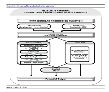
Source Annex 3 of the Ageing report 2024 – Underlying Assumptions and Projection Methodologies
The public spending multiplier and the evolution of GDP towards potential GDP
In the short term, in this model, GDP growth is determined by the Commission’s latest forecast, and then partly by the potential growth calculated by the production function presented above. The growth forecast for the adjustment period also takes into account a multiplier effect of public spending. multiplier effect of public spending equal to 0.75 times the change in the primary budget balance.
In other words, beyond the short-term forecast period 28 forecast growth is equal to potential growth less three-quarters of the required change in the budget balance, widening the gap between forecast and potential GDP while leaving potential GDP unchanged.
At the end of the adjustment period, it is assumed that theoutput gap 29 will be eliminated in no more than three years. The assumption is therefore that there is no lasting effect of fiscal policy on growth. In addition, the fiscal multiplier (i.e. the impact of a variation in the structural deficit on GDP) is estimated at 0.75, regardless of the country, the fiscal instrument used (taxes, investment, public consumption), or the economic situation.
These assumptions run counter to numerous studies, including those of the IMF.30
Inflation, interest rates and public debt trends
The inflation rate adopted for the projection period is 2%, the target used as a guide and reference by the European Central Bank. This 2% figure is debatable.
For interest rates, economists use country-specific assumptions. For the European Union as a whole, the average cost of refinancing public debt in the long term (from 2046 onwards…) is equal to 2% plus the inflation rate – to which a target of 2% is assigned – i.e. an interest rate of 4%. 31 In the medium/long term, the cost of refinancing public debt converges for all countries to this conventional level of 4%.
With a long-term real GDP growth rate of 1.3% (or 3.3% including inflation), we find ourselves in the situation described in section 2.2, where the primary balance stabilizing (or reducing) the debt-to-GDP ratio must be positive and greater than around 1% of GDP. This is also true for almost all EU countries, as the reader will see from the tables on pages 9 and 73 of the Ageing Report 2024 .
The Commission’s debt sustainability analyses, which have been carried out for several years now 32 are one of the instruments of multilateral surveillance. The 2024 reform introduced them into the legislative corpus 33 and thus made them prescriptive, based on arbitrary sustainability criteria (the 60% and 3% limits). Under the new legislation, the “calculations” made by the Commission are to be used to determine the norm, i.e. the budgetary trajectory to be respected by the Member State.
Modeling the evolution of public debt
The following equation from the Debt sustainability Monitor 2023 (Annex 3) describes the evolution of a stock (of debt) as a function of a flow (the deficit) and the key parameters of the interest rate on the debt and the growth rate (since the reasoning is always based on the ratio to GDP).
We reproduce this equation below, as it appears in the Commission’s document.
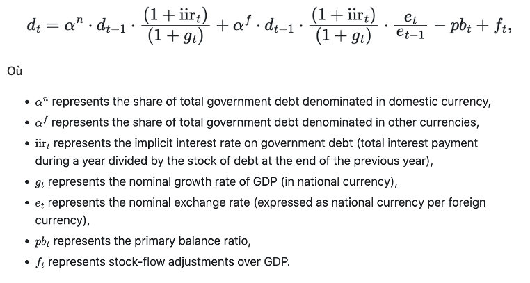
It illustrates the extent to which all the methodological documents used by the Commission’s departments are full of equations of this type. These equations contain assumptions that reflect ideological judgments or biases (see section 5.1 on the production function, for example). Debates on subjects as essential as a government’s budgetary trajectory are therefore confiscated by the small circle of economists who know how to read them and interpret them critically (and have the time to do so). As the biases adopted are invisible to the average person, they cannot be – and are not – discussed.
The introduction of alternative scenarios and hazards
In the 2024 version of the budgetary rules, and in line with the debt sustainability analysis method, the Commission carries out “stress tests” on three deterministic scenarios 34 alternative to the baseline scenario (which determines the minimum budgetary adjustment consistent with the objectives of the Stability Pact).
- Scenario “Primary Structural Balance (PSB) smaller than required”: PSB is assumed to be reduced by 0.5% of GDP in total, with a reduction of 0.25% each year for the first two years, and to remain at this level thereafter.
- Unfavorable r-g”scenario: the spread between interest rates and growth rates is assumed to increase permanently by 1 percentage point.
- Financial stress” scenario: market interest rates are assumed to rise temporarily for one year by 1 percentage point, plus a risk premium for highly indebted countries.
These tests and random shocks 35 are taken into account 36 in the final budget scenario, which is designed to :
- that these less favourable scenarios do not call into question compliance with the budgetary objectives set for the deficit and debt;
- that these objectives are met for 70% of random shocks to the main parameters simulated.
Summary
The following graph illustrates the overall reasoning behind a numerical example.
Illustrative example of the reference trajectory respecting the debt sustainability criterion
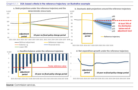
Source Debt Sustainability Monitor 2023, page 112
On these graphs (which run until 2038, which is already absurd), we can see the simulations carried out on the key variables of the reasoning: public debt (graphs a and b), budget balance (graph c), net public expenditure (graph d); as well as the four-year adjustment period which is supposed to put the variables back on the right trajectory.
The limits of these rules
The budgetary rules we have just presented and explained are essential in economic terms, and provide a framework for many public policy decisions, far more than is generally understood. Let’s take two well-known examples:
- the measures taken to tighten unemployment conditions are seen by many economists as likely to increase potential growth and thus facilitate compliance with these rules;
- public investments (including those required for the ecological transition) would, on the contrary, make it more difficult to comply with budgetary rules. These are the conclusions of the report The implications of public investment for debt sustainability published by DG ECFIN in early 2024. 37
However, these rules suffer from a number of fatal flaws.
- They specify how to comply (by Member States) and enforce (by the Commission) ratios (3% and 60%) that have no economic rationale.
- They are particularly opaque and difficult to understand, and therefore beyond any democratic deliberation.
- In fact, they give excessive discretionary and decision-making power to national (Ministries of Finance) and European (DG ECFIN) bureaucracies. More specifically, in France, a very small caste 38 has power over the trade-offs that need to be made to comply with these rules, or to depart from them in an acceptable manner.
- The budgetary procedure remains profoundly asymmetrical and does not loop back to the European macroeconomic level: all countries are encouraged, or even forced, to reduce public spending. None, even those who could do so without any problem under the existing rules, are encouraged to spend more. The macroeconomic effect is therefore very likely to be recessionary for the EU as a whole. This really isn’t the time, given the scale of the climate investments required, the war on Europe’s doorstep, the risk of a strategic pivot from the USA to China, and the increasingly intense economic war.
- They are based on the use of non-measurable concepts of questionable evaluation (potential GDP, structural deficit, NAIRU, etc.).
- They are based on flimsy macroeconomic models that do not take into account the effects of climate change.
- They include a low public spending multiplier of 0.75, constant for all countries, and a constant 3-year period of convergence of GDP towards potential GDP, assumptions that are largely arbitrary and highly penalizing from an economic point of view, in a context where China and the United States are exerting ruthless competition on European economies, particularly in terms of green industry.
- They are based on strong assumptions about inflation rates, interest rates and monetary policy, which are highly debatable.
- Several variables, which are difficult to estimate, such as those we have highlighted in this sheet, have substantial effects on the results obtained, despite the “robustness” tests; consequently, all the work done is in fact not robust.
- They make no difference to the nature of public spending (investment versus current expenditure, etc.), and fail to take into account the effects of climate change and the collapse of biodiversity on European economies, or the urgent and essential need for spending and investment to reduce impacts and adapt, as far as possible, to changes already underway.
- In this respect, the three-year adjustment period is highly problematic, since it is now, and in any case between now and 2030, that we need to accelerate and amplify the investments required to combat climate change and adapt to the effects already underway.
Find out more
- Our detailed fact sheet on European economic governance.
- The link to the codes used to “run” the models used by the Commission, provided by the Bruegel think tank.
- The 4-part series on the importance of linking fiscal governance to environment/climate/energy governance, Greentervention, 2023.
- Philipp Heimberger et al, Debt Sustainability Analysis in Reformed EU Fiscal Rules: The Effect of Fiscal Consolidation on Growth and Public Debt Ratios, Intereconomics, 2024
- Lennard Weslau, the Bruegel expert who published the codes, explains in a thread on X (ex twitter) the difference between the old and new rules.
- Note on the importance of reflecting on the principles of coordinating budgetary policies beyond accounting rules, Greentervention, 2022.
- With the publication of Regulation 2024/1263 on multilateral budgetary surveillance, Regulation 2024/1264 on the correction of excessive deficits and Directive 2024/1265 on the budgetary framework for European States. ↩︎
- The main document is the Debt Sustainability Monitor 2023, (298 pages, see in particular chapters I.2 and II.1 and, for the arithmetic, appendix 3, P. 131). This document refers to methodologies developed in Ageing Report. Underlying Assumptions and Projection Methodologies (2024, 224 pages) and in the methodological report of the Output gap working group (2021, 62 pages). ↩︎
- The finance departments of the 27 EU member states and those of the Commission’s Directorate-General for Economic and Financial Affairs (DG ECFIN). ↩︎
- Barring exceptional situations such as epidemics or major financial crises… ↩︎
- Guy Abeille was a chargé de mission at the Ministry of Finance under the presidency of Valéry Giscard d’Estaing and at the beginning of that of François Mitterrand. Read his account La petite histoire des 3 % du PIB, published in issue 40 of Variances. ↩︎
- In 2023, the average public debt of European Union countries was 82%, with 13 countries exceeding 60%. On this subject, see the received idea Beyond a certain level, public debt (in relation to GDP) would be unsustainable in our module on public debt and deficit. ↩︎
- What Is Debt Sustainability and Why Does It Matter?IMF, 2009 ↩︎
- For a more detailed version, see our European Economic Governance fact sheet, parts 2 and 3. ↩︎
- The crises at the turn of the 2010s highlighted the inadequacy of budgetary surveillance: other macroeconomic imbalances, such as excessive private debt or a balance of payments imbalance, can destabilize the EU economy. The economic coordination measures previously focused on budgetary surveillance were therefore supplemented in 2011 by the surveillance of macroeconomic imbalances. See Regulation 1176/2011 and our European Economic Governance fact sheet ( part 4). ↩︎
- How has the macroeconomic imbalances procedure worked in practice to improve the resilience of the euro area? Bruegel, 2020. ↩︎
- This is public spending MINUS interest charges; the cyclical variation in unemployment spending; the variation in tax revenues due to discretionary measures (for example, an increase in revenues linked to a rise in the tax rate is deducted from net public spending); spending financed by European funding; one-off or temporary measures. ↩︎
- Which can be extended up to 7 years if the country commits to an ambitious investment and reform program improving “potential growth and resilience potential” and contributing to the achievement of the Union’s objectives. ↩︎
- There is a minimal difference between the deficit and the increase in debt: acquisitions and disposals of non-financial assets are recorded in the national accounts as capital expenditure (negative in the case of disposals). They therefore have an impact on the public deficit equal to their amount, and do not create a difference between the deficit and the change in debt over a given period. This difference does not change the reasoning: the essential point is to understand that the public deficit is a cash requirement and not an accounting deficit in the calculation of which investments have been amortized. ↩︎
- See the snowball effect fact sheet on the Fipeco website. ↩︎
- More specifically within DG ECFIN. ↩︎
- The unemployment rate used is therefore the ” NAIRU “(Non-Accelerating Inflation Rate of Unemployment ), which would be compatible with a stable inflation rate. This NAIRU is not directly observable, so its estimation relies on questionable econometric tests. See our module on labor and unemployment. ↩︎
- Events that are set to become increasingly frequent as a result of ecological crises… ↩︎
- That is, excluding exceptional circumstances such as COVID or the 2008-2009 crisis. ↩︎
- See details of the excessive deficit procedure in our European economic governance fact sheet , section 3.2. ↩︎
- See p. 113 of the Debt Sustainability Report 2023. This convention takes into account the automatic increase in revenues assumed to be proportional in the medium term to that of potential GDP, and the variation in net public spending adjusted for cyclical variations and exceptional expenditure, as well as discretionary measures affecting revenues. ↩︎
- See the Excel file provided with the Ageing report 2024 – Underlying Assumptions and Projection Methodologies report, which details the demographic and macroeconomic assumptions used to update long-term budget projections. ↩︎
- See Appendix 3 of the Ageing report 2024 – Underlying Assumptions and Projection Methodologies, which details the underlying macroeconomic model. ↩︎
- The Cobb-Douglas function is a function used in economics as a production function model, i.e. to express the relationship between factors of production and quantity produced. For more information, see the Wikipedia entry on the subject. ↩︎
- To find out more about how economists model GDP growth and Total Factor Productivity, see the Essential ” GDP growth is not explained by the most widely used macroeconomic models ” in the module on GDP, growth and planetary limits. ↩︎
- See also The Production Function Methodology for Calculating Potential Growth Rates & Output Gaps, 2014 and the Commission working group dedicated to estimating potential GDP. ↩︎
- See, for example, this article by Bernard Guerrien, Aggregate production function and ideology , 2017. ↩︎
- See our fact sheet on supply-side policies. ↩︎
- Short-term forecasts for 2025 date from spring 2024, and the first for 2026 from autumn 2024. ↩︎
- Theoutput gap is the difference between potential and actual GDP. ↩︎
- See in particular Fiscal consolidation – Taking stock of success factor, IMF, 2023 and Getting into the NittyGritty of Fiscal Multipliers: Small Details, Big Impacts, IMF 2023. ↩︎
- These projections are based on an agreement reached in 2009 (i.e. before the massive fall in real rates of the last decade) by the Economic Policy Committee’s Working Group on Ageing Populations and Sustainability (AWG), and maintained as part of the preparation of subsequent Ageing Reports, as well as a few additional assumptions. ↩︎
- Known by their acronym ESA (Eu debt Sustainability Analysis). ↩︎
- In particular in Regulation (EU) 2024/1263, which structures the preventive arm of the Stability and Growth Pact. ↩︎
- A scenario is said to be deterministic when each variable in the model is assigned only one value per period determined by the model. It is random when the model assigns each variable a distribution of possible values with associated probabilities of occurrence. ↩︎
- Random shocks are also tested using a classical Monte Carlo method. ↩︎
- See Debt Sustainability Monitor 2023, page 11. ↩︎
- See Ollivier Bodin’s analysis on the Chroniques de l’Anthropocène blog. ↩︎
- These include current or former Directors General of the Treasury or Public Finance, such as Emmanuel Moulin, Bertrand Dumont and Jérôme Fournel, who are or have been in key political positions (Chief of Staff to the Prime Minister or Minister of Finance). ↩︎