
This text has been translated by a machine and has not been reviewed by a human yet. Apologies for any errors or approximations – do not hesitate to send us a message if you spot some!
Numerous “laws” have been proposed by economists since the founding work of the first economists in the 18th century. These “laws” or “theorems” have been imagined in the image of physical laws and mathematical theorems, while the very idea of law is debated in the economic field.
Unlike physics1 or biology, economists can’t conduct controlled experiments to verify their theories.2 For example, he can observe a correlation between rising unemployment and other variables (inflation, foreign trade trends, etc.), and put forward explanatory phenomena, but he cannot deduce a precise and always verified causal link – i.e. a law – because it is not possible to test the influence of this or that cause “all other things being equal”.3
As we’ll see in this fact sheet, “the law of supply and demand”, “Say’s Law” and “the law of diminishing returns” are not laws. This name is dangerous, because it suggests that they are universal and permanent, and therefore intangible. Simple statements that may prove to be true in very specific situations then become dogmas. Dogmas that are further reinforced by the fact that the majority of these “laws” are based on a more or less sophisticated mathematical demonstration that gives them an appearance of solidity that they do not have.
In this fact sheet, we’ll list the most important ones, explain in simple terms how they’ve been “proven”, and summarize the main criticisms that can be levelled at them.
The absence of “universal economic laws” does not preclude the formulation of scientifically valid statements
The absence of “economic laws” does not mean that everything in economics is necessarily relative, that everything is debatable and that nothing can be affirmed. On the contrary, the economic sphere today is far too structuring of social and political life to be content with a “relativistic” approach.
It is possible to put forward facts and statements which, while not physical laws, are scientifically sound, and which very often contradict the most widespread analyses, particularly as these take no account of the physical and living foundations on which the economy rests. Not to do so is to allow current dogmas to persist, in the absence of a structured alternative.
These facts and statements fall into three broad categories:
- those linked to the fact that the economic system is part of a physical and living world, which affects it and on which it has an impact.
- those of an accounting nature (these are often tautological or purely descriptive truths). For example: every debt has a counterpart debt; one man’s income is another man’s expenditure; reducing public spending means reducing the income of those (companies or households) who used to benefit from it; money is now created by banks through a simple accounting entry.
- those based on empirical regularities over long periods. For example, it is a proven fact that the number of hours worked in France has been falling steadily for two centuries, and this trend is clearly correlated with the mechanization of work. Or again: the share of wages in GDP in France was more or less constant from 1945 to the 1980s, and has been falling ever since.
From these empirical regularities, the economist can detect major “trends” at different moments in history or in different societies, and draw lessons from them. They are not, however, “laws”, intangible, universal rules. Economic life takes place in a natural and social environment, the product of history, institutions and legal frameworks. That’s why it’s always important to place great economic ideas in the historical context in which they emerged.
The “law “ of supply and demand
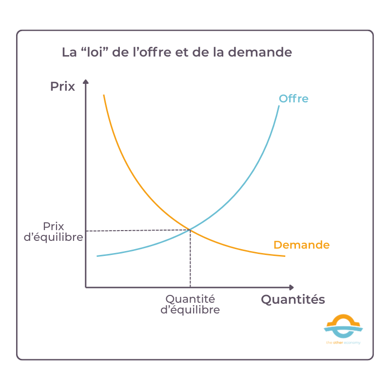
This law states that when the supply of a good or service increases while demand remains constant, the price decreases, and vice versa. Prices would thus be set by the confrontation between supply and demand for the good or service concerned.4the equilibrium price being reached when demand equals supply.
It is taught as the ABC of economics. It’s quite intuitive: we tend to buy a cheaper product more easily or in greater quantity than another (for the same quality). This is the case, for example, during sales. Conversely, the more expensive a product, the more careful we are to limit consumption.
Mathematically, this law can be demonstrated using a very simple result. Supply of a good is represented by an increasing function of price, and demand by a decreasing function. These two curves have a point of intersection that defines the price where supply equals demand.
Simplified diagram of the “law” of supply and demand
This law is false in its generality
The economists behind this theory themselves identified the existence of essential goods (known as Giffen goods) whose demand increases when their price rises in a context of generally rising prices. In this case, populations for whom this good represents a significant proportion of income will be forced to forego other types of goods, and will increase their consumption of this good to compensate.
There are, however, a few exceptions. For example, as Sir R. Giffen has pointed out, a rise in the price of bread drains the resources of poor working-class families to such an extent, and so raises the utility-limit of money for them, that they are obliged to reduce their consumption of the most expensive meat and flour products: and, bread still being the cheapest food they can consume, far from consuming less, they consume more.
Alfred Marshall, Principle of Political Economy, 1890
Luxury goods are another example: their demand can rise with their price, as they serve as status symbols.
Prices are based above all on production costs: these set a floor price below which, even with insufficient demand, a company cannot sustainably fall without going bankrupt. For the proponents of the law of supply and demand, this is a rather healthy consequence, since it would enable under-performing companies to be weeded out.
The law of supply and demand does not apply in the case of speculation: for a financial product, for example, the higher the price, the greater the demand (momentum logic). This is also what happens on the commodities markets.
Finally, there are single-price products, such as books in France. According to theory, having a fixed price should translate into fixed demand (to which supply should adjust). But this is clearly not the case.
The mathematical formulation of the law is a perilous exercise when confronted with reality.
More fundamentally, as soon as we consider formulating this “law” in a mathematically rigorous way, the difficulties pile up and all that’s left is a vague slogan, the consequences of which in terms of market equilibrium are by no means self-evident, as we’ll see when we look at the “law” of general equilibrium.
Here are some of the difficulties.
- How is the market for the goods and services concerned precisely defined?
- Which products are concerned? (e.g. all bakery products? only breads? if so, which breads?…).
- What quality are they? (A pastry sold by a “Meilleur ouvrier de France” craftsman does not compete with an industrial pastry, which may cost 10 times less… Does a cow’s yoghurt with fruit compete with a soy yoghurt? etc.).
- In what geographical area are we thinking? (in a given city? a region? a country?)
- Who are the “suppliers” to be considered (producers, intermediaries, end sellers)?
- Which customers should be considered (end customers? wholesalers, if applicable? all types of distribution outlets?)
- Over what period of time (some products, such as in the digital sector, change very quickly… As a result, do the form of the law and its parameters change every year?
- How can we mathematically formulate the law of supply and demand for the market thus specified?
- How do you check its validity?
- Can we determine the points on the supply and demand curve? You need quantities offered, envisaged demands and the prices that would result from this “confrontation”, whereas in fact the only information available at any given moment is the price of a product and the quantities sold…
The “law” of general equilibrium
The law of supply and demand is, as we’ve just seen, a rather vague theory. Following Léon Walras5economists attempted to represent markets mathematically, and to show that they could spontaneously lead to a “general equilibrium”, a situation in which, on all markets, supply and demand would equalize thanks to an equilibrium price.
Kenneth Arrow and Gérard Debreu are credited with having rigorously formalized the theory of general equilibrium in an article published in 1959 with the revealing title: The Existence of an Equilibrium for a Competitive Economy(Econometrica, 1954).6). It is often said that this article effectively demonstrates the existence of such an equilibrium.
As is always the case in mathematical economics, the demonstration involves numerous simplifications and assumptions. Here are some of the most salient and decisive in the demonstration carried out by Arrow and Debreu:
Economic agents are assumed to be “rational”.
This assumption is not in line with reality, as numerous empirical studies have shown, and as common sense teaches us directly without the need for demonstration. To find out more about the concept of rationality in economics, see our Infosheet Rationality in homo economicus: an unfounded hypothesis.
Their preferences are represented by a “utility function” assumed to be convex
Convexity of preferences means, in economic terms, that consumers value diversity and appreciate consuming moderate quantities of different goods, rather than concentrating on a single good. This hypothesis is consistent with the principle of diminishingmarginal utility: the more of a good consumed, the lower the additional utility provided by an additional unit of that good. So diversifying consumption increases total utility.
The question is whether this hypothesis is confirmed empirically…
Consumer preferences are assumed to be independent of those of others
This is obviously contrary to everything observed by psychologists, sociologists and anthropologists, for whom desire is mimetic. It also contradicts the methods of marketing and advertising, which aim precisely to create consumer desire based on the supposed consumption of a social model or reference.
Competition is assumed to be perfect
One of the necessary conditions for a perfectly competitive market is market atomicity: there are a large number of suppliers and demanders, and all these economic agents are considered “price takers”, meaning that they don’t set prices – they take them, wherever they come from. This last assumption is often presented as valid in the case of “small” agents, whose individual offers and demands drown in the mass. In reality, there are many situations of monopoly and oligopoly. Moreover, the central question of who sets prices is left unanswered. Whether agents are few in number or not, someone has to do it. This mystery remains unanswered, as modeling does not explain how prices are formed.
Returns are assumed to be decreasing
In reality, returns are increasing in many sectors of the economy, and the limits of the law of diminishing returns are explained below.
The market system is assumed to be complete
All present and future assets7 are assumed to be traded on a market and therefore to have a price. This assumption is obviously false.
The decisions of one agent do not directly affect the “utility” or production function of other agents: there are no “externalities”.
The term externality refers to the positive or negative repercussions of an economic agent’s activity on other agents, without any monetary compensation. For example, the discharges of a factory polluting a river have negative effects on water users, without the company having to pay anything for this. Clearly, economic activities have a variety of potentially considerable effects on humans and nature, without giving rise to a market exchange. The assumption that there are no externalities is obviously false.
Market failures: adapting theory to reality
Neoclassical economists8 generally recognize that these assumptions are not respected in the real world, and use the expression “market failure”.
For example, an environmental externality is a market failure. In this case, the same economists recommend “internalizing” it (reintroducing it into the market) by giving it a price (via an environmental tax such as the carbon tax, or a quota market mechanism such as the SEQE-EU European carbon market).
All these discrepancies between theory and fact show that the theory’s conclusions have no empirical basis.
Find out more
- ” Market equilibrium: a myth that lives on despite the facts ” in The Other Economy’s Market, prices and competition module.
- ” The capacity of markets to self-regulate to an optimal situation has been scientifically demonstrated ” in the Market, Prices and Competition module of The Other Economy .
- Fact sheet The rationality of homo economicus: an unfounded hypothesis, on The Other Economy
- Fact sheet The utility function in economics: definition and problems, on The Other Economy
- What is perfect competition?Bernard Guerrien, 2017
- Neoclassical equilibrium, on Christophe Darmangeat’s Introduction to economics site
Financial markets are efficient
The “demonstration” of the efficiency of financial markets earned American economist Eugene Fama the 2013 “Nobel Prize in Economics”.9 which he shared with another economist, Robert Shiller, who… disputes – and rightly so – this idea, claiming instead that markets are exuberant and irrational.10
Here too, the idea has been much talked about.11 Mathematician Nicolas Bouleau has produced a remarkable critical analysis, focusing on semantics and the use of modeling.
In this way, we can see an attempt to link the economic notion of efficiency, which can only mean the “right” allocation of resources (capital, investment) to avoid waste, to mathematical formalizations of random processes (martingales or semi-martingales for discounted prices, Markov processes, filtering).
Nicolas Bouleau, Critique de l’efficience des marchés financiers, 2013
Say’s Law
According to this law, supply creates its own demand. In other words, the total output of an economy generates sufficient income to buy that output. It’s true that companies producing goods or services spend the money they receive, which is income for employees, suppliers, bankers, government bodies and shareholders.
But the apparent tautology of this law is false, because it’s not production that generates income, but sales. The economic purchasing power generated by companies is equal to their sales, not their production. There may be unsold products (and therefore inventories) which are not income for companies, and which they cannot spend again. This is so true that capitalism has experienced so-called crises of overproduction, the most famous of which was the 1929 crisis, which was in fact a crisis of underselling. In 1929, companies unable to sell what they had produced went bankrupt, and so did the banks.
To find out more, see The Other Economy Fact Sheet: Putting an end to Say’s law, or the law of opportunities.
Ricardian equivalence and the crowding-out effect
The English economist David Ricardo was the first to assert that there would be an equivalence between an increase in public debt today and a future increase in the taxes levied by the State to repay this debt and pay the interest. For example, according to him, it would be equivalent for a State wishing to finance a war to raise a new tax or to issue debt securities.
Economist Robert J. Barro formulated this idea mathematically in a landmark article12 in 1974. His demonstration was further refined by James M. Buchanan in 1976. 13
For these authors (and the entire school of thought that follows them, the ” new classical economists “), fiscal stimulus policies are ineffective. According to them, economic agents anticipate a future tax increase when faced with a fiscal stimulus. As a result, they adjust their level of savings (and hence investment) and consumption to neutralize the fiscal policy. Public borrowing, like taxation, therefore has a crowding-out effect on private investment.
The same conclusion can be drawn in the case of monetary financing (due to the “invariance principle” posited by Sargent and Wallace – see next point). Agents anticipate the regular issue of new money and the erosion of their savings by inflation. They therefore save to reconstitute the real value of their balances. There is therefore no multiplier effect from fiscal policy.14 on aggregate demand, contrary to the approach developed by the English economist John Maynard Keynes15 and his successors.
As always, the mathematical models used are based on numerous simplifications. Without going into a detailed analysis here, let’s just mention the most notable ones:
- The economy is represented by an ultra-simplifiedgeneral equilibrium model (based on a highly questionable theory, as seen above), with a production function such that wages are equal to the marginal productivity of labor.16 and capital is remunerated at a single interest rate.
- Economic agents are assumed to be capable of “rational anticipation”. They maximize an intertemporal utility function to infinity (which means they are altruistic towards their descendants, whom they consider to have the same interest as themselves).
- Financial markets are assumed to be perfect (freely accessible, transparent, with no transaction costs, with a very large number of agents, assumed to be rational, with no regulatory constraints).
- Taxes are assumed not to affect consumption or savings choices.
- Public spending is assumed to be neutral, i.e. incapable of modifying “real” economic data, and therefore of having an impact on employment or growth.
The theory of rational expectations
Introduced by American economist John Muth in 196117this theory postulates that economic agents are capable of analyzing and anticipating as best they can the situation and events in the world around them, in order to make the best decisions to maximize their personal interest (their “utility”). It is, to use Gaël Giraud’s expression18, “ the ability to predict the future! To be more precise: all future variables are assumed to follow probabilistic laws known to everyone, and each agent is assumed to maximize the measure of his or her “happiness” (or profit) by anticipating exactly the mean (probabilistic expectation) of these random variables. “. Economic agents are therefore able to anticipate the consequences of economic policies initiated by governments. The American economist Robert Lucas developed this idea by asserting that agents immediately adjust their behavior to economic policies, perfectly anticipating their impact on currency and price variations. 19
This theory is obviously completely false. Citizens and companies do, of course, have capacities for anticipation, but they are much more limited than those attributed to them by the theory. Nevertheless, the theory has played an important role in criticizing public policy and the ability of governments to intervene effectively in the economy, as shown by Olivier Blanchard and Daniel Cohen, for example, for whom the theory of rational expectations is considered by ” most macro economists as the best possible hypothesis for evaluating an economic policy measure “.20
For a mathematical formalization of this theory, see Gabriel Desgrange’s article Équilibres et anticipations, 2017.
As these assumptions are empirically unfounded, the conclusions are questionable, to say the least. In any case, they cannot be considered as the result of a demonstration.
Following on from this work, empirical studies have sought to identify so-called “Ricardian” household behavior (i.e., the consumption-savings trade-off that Robert Barro attributes to all agents). They do not allow us to draw any clear conclusions, which is to say that, in its generality, the hypothesis that households are Ricardian is unfounded.
Numerous studies have addressed the question of the effect of public spending and the validation of the fiscal multiplier. Their conclusions confirm the existence of this mechanism, the controversies surrounding its quantitative evaluation and the conditions that make it lower or higher.
To find out more, visit the Ricardian equivalence pages on Wikipedia and the Melchior website.
Sargent and Wallace’s “principle” of invariance (or monetary neutrality)
According to American economists Thomas Sargent and Neil Wallace, monetary policy cannot be effective in the short term. Their “demonstrative” paper, published in 197521was based on a mathematical model and the idea that ” monetary policy, if systematic and consistent, would be anticipated by economic agents“.22 which would neutralize its effects. There would therefore be no real effect on the economy, only an effect on nominal values. “.23 This means that prices can change, but not the quantities traded.
In the 1970s, central banks adopted monetary neutrality as a cardinal principle. It is one of the foundations of the European treaties which defined the central bank’s primary mandate as the fight against inflation. According to the principle of invariance, money creation is supposed to have no effect on the real economy, but only on prices. As a result, it would disrupt the smooth functioning of markets and, in particular, the proper allocation of savings.
Like Ricardian equivalence, this principle is based on the theory of rational expectations, which is highly debatable and has no empirical basis. But it is also based on a dogma and a double belief. The dogma is the monetarist belief that inflation is exclusively monetary in origin, and that an increase in the money supply will always result in inflation. The belief is twofold: it is the belief of these economists in this dogma, and in the idea that this dogma would be shared by citizens. In their eyes, if citizens are supposed to be rational, they are supposed to share the theory adopted by these economists….
Without going into further analytical considerations, it is not difficult to give examples of cases where monetary policy has been anything but neutral.
Let’s take a look at monetary policy (and the famous Treasury circuit) in France during Reconstruction24quantitative easing operations in the 2010s, and, conversely, periods of deflation, such as Brüning’s Germany, or the 1929 crisis, when the failure of monetary authorities to intervene fuelled crises.
To find out more about this topic, see the Money module and the Inflation and Money fact sheet on The Other Economy.
Haavelmo’s “theorem
The Norwegian economist Haavelmo (a Keynesian) sought to demonstrate in an article published in 194525 that an increase in public spending, entirely financed by an increase in taxation, would boost economic activity. The demonstration is very simple (see box below) and is based on the assumption that the public spending multiplier (ratio of GDP increase to spending increase) is greater than the tax multiplier (ratio of GDP increase to tax decrease).
The rationale behind this hypothesis is as follows: increasing public spending can raise aggregate demand by the same amount, while raising taxes only reduces demand for that part of the additional levy that would not have been saved. In other words, public spending would be entirely transformed into income, while tax cuts can be saved, with no effect on activity.
This demonstration is, however, questionable due to a number of simplifications.
- The reasoning is based on a closed economy, with open borders creating “leakage” of activity and a possible increase in the trade deficit.
- The model’s central parameter, the marginal propensity to consume, is very difficult to know, and can only be assessed using econometric models and tests.26
- An increase in taxation can have negative effects on economic activity by reducing the return on investment or the return on labor, with a consequent drop in the demand and/or supply of labor.
An empirical study of 200 “consolidation” experiments carried out in 16 countries over the period 1970-201427 shows that, for the same tax yield, “consolidations” involving a reduction in spending have significantly lower adverse effects on activity than those involving an increase in taxation.
In short, if Haavelmo is pointing to an important argument in the conduct of fiscal and budgetary policies, it is an exaggeration to use the term theorem, which could give a character of mathematical truth to a debatable subject.
Demonstrating Haavelmo’s theorem
Let’s start with a balanced budget, G = T (G = expenditure, T = taxes).
The State decides to increase its budget, while remaining in balance: G + ΔG = T + ΔT, and therefore ΔG = ΔT.
By definition, the evolution of output Y (GDP ) is ΔY = kG.ΔG + kT.ΔT, where kG and kT are the public spending multiplier and the tax multiplier, respectively.
Since kG = 1 / (1 – c) and kT = – c / (1 – c), (c =marginal propensity to consume),
we have :
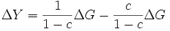
or :
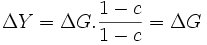
This means that the increase in public spending has led to an increase in GDP of the same amount.
The cost-share “theorem” assessing the weight of energy in GDP
Taught in all microeconomics courses, the cost-share theorem is important because it suggests that the sensitivity (or, in other words, the dependence) of GDP on a production factor is equal to the share of GDP allocated to that production factor.
So, since energy represents a very small proportion of GDP, the latter would not be very dependent on it. This is obviously false for energy, and even more so for water and food. Shortages of energy, water or food have considerable social and economic consequences that reverberate throughout the economy, far beyond the share of these economic sectors as counted in GDP.
More rigorously, according to the cost-share theorem, there is equality between the share of the remuneration of a factor of production and the share of the remuneration of a factor of production.28 in the cost of production and the elasticity29 of production to this factor. For example, if the elasticity of production to the “labor factor” is 0.6 (an increase in the quantity of labor of 100 increases production by 60), the remuneration of this factor must be 60% of the cost of production. We can also say that the remuneration of a factor of production is equal to its “marginal productivity”.
The reasoning can be done the other way round. If the remuneration of a factor of production is X% of production, then production is elastic to this factor at a rate of X%. The intuitive underlying idea is that if one factor is paid more than another, it is because that factor is a relatively greater contributor to output.
Economists applying this “theorem” deduce that variations in energy production have little impact on GDP, since its share of remuneration in GDP (around 10% maximum) is low.
Find out more
- Can there be growth without energy? on The Other Economy
- Video Growth & energy: the economists’ mistake? on Eu?reka’s Youtube channel
- Gaël Giraud, Zeynep Kahraman, How Dependent is Growth from Primary Energy? The Dependency ratio of Energy in 33 Countries (1970-2011) , 2014.
Okun’s “law” on the link between GDP growth and unemployment
That GDP growth drives employment is one of the most widely held beliefs among economists. American economist Arthur Okun formulated this belief as a “law” in an article in 1962 and a book in 1970. 30
This law has no theoretical basis31 and simply describes an empirical linear relationship between the rate of GDP growth and changes in the unemployment rate.
Strictly speaking, it makes no sense to say that a rise in GDP will reduce the unemployment rate: GDP is a concept, just like the unemployment rate. Moreover, both GDP and the unemployment rate are largely conventional concepts.32 A low unemployment rate, for example, is not synonymous with full employment.33 Finally, from an empirical point of view, what can be demonstrated are correlations, not causal links.
This “law” can be written very simply: Y = c U + d , (Y is GDP; U is the unemployment rate; c and d are coefficients to be determined).
It can also be written in the following way, which is how Okun presented it:
ΔUt = β x (GDPt-GDPt*), for a year t, where ΔUt is the variation in the unemployment rate, GDPt the GDP growth rate, GDPt* the economic growth threshold above which the unemployment rate falls and β the “Okun coefficient” (β < 0, this is the elasticity of unemployment to GDP).
Over the period observed, Okun found a β rate of -0.3 for the United States, meaning that a 1% fall in unemployment corresponds to a 3% rise in GDP. This law can therefore be used in practice in two ways: it tells us what the minimum growth rate is for growth to “create” jobs and, if this floor is exceeded, what impact it will have on employment.
Numerous econometric studies have been carried out to validate this law and determine the Okun coefficient. They show that this coefficient varies from country to country and from period to period. For example, according to an IMF study34 published in 2013, it varies between -0.25 and -0.55. In his doctoral thesis35economist Gaëtan Stephan carried out a meta-analysis of 28 articles on Okun’s law published between 1989 and 2009. He found 269 Okun coefficients ranging from -3.22 to 0.17. For France, a study36 for the period 1963-1978 estimated it at -0.2.
Finally, this law says nothing about the mechanisms involved (stimulating growth or the employment rate) or the nature of the jobs created.
What does this mean? That this “law” is not, of course, a law in the physical sense of the term. It can provide, for a given country and a given year, a sort of “wet-finger” estimate that can, at best, be used to check more elaborate estimates based on large economic models: what might be the variation in unemployment next year if GDP varies in such and such a way? On the other hand, it in no way provides a valid rule for the long term, in any country.
Phillips’ law on the link between unemployment and inflation
In 1958, economist Alban W. Phillips published an article37 in which he demonstrated an inverse relationship between the rate of change in nominal wages and the unemployment rate in the UK over the period 1861-1957: the higher the unemployment rate, the lower the increase in wages.
The underlying reasoning is fairly intuitive: if unemployment is high, workers are prepared to accept lower-paid jobs for fear of unemployment. Conversely, in periods of low unemployment, they have a favorable balance of power to negotiate higher wages.
This curve is better known in a slightly different form: that of the link between unemployment and inflation. Unemployment and inflation are said to be negatively correlated.
There are two reasons for this:
- As labour costs are generally the most important production cost for companies, any increase in these costs can be passed on to sales prices;
- Economists consider the unemployment rate to be an indicator of the state of aggregate demand in the economy (this is linked to Okun’s law). The lower the unemployment rate, the more likely it is that the economy is in “good health”, and that demand for consumer and producer goods (investment) is relatively high. This high demand can create inflationary pressures if supply fails to keep pace.
The Phillips curve is the observation of a correlation between two indicators (unemployment rate and inflation), the construction of which is based on conventions. For example, as already mentioned for Okun’s law, a low unemployment rate is not necessarily an indicator of full employment.
Beyond the statistical work and these limitations, we can say a word about the theoretical challenge posed by this curve. According to Keynesians, who tend to support the existence of this correlation, wages are not the result of a law (which would equalize them to the marginal productivity of labor). They see the Phillips curve as a materialization of wage determination, which is determined by a balance of power: wages are linked to tensions on the labour market, and to the distributional stakes between wages, profits and prices. It’s hard not to agree with them, which doesn’t prevent us from discussing the existence of a mathematical “law” fixing the correlation between the unemployment rate and wage levels.
To find out more, see The Phillips curve: the link between unemployment and inflation on The Other Economy.
Ricardo’s “theorem” of comparative advantage
We owe David Ricardo an argument in favor of international trade, known as the comparative advantage theorem, as opposed to the “absolute advantage” theorem formulated by Adam Smith a few decades earlier.
In simple terms, according to this “theorem”, any country would gain from specializing in the production of goods for which its comparative advantage is the highest, i.e., whose relative costs are the lowest, and from buying abroad the goods it does not produce. This is an argument in favor of free trade: all countries stand to gain from free trade by specializing.
This theorem is usually “demonstrated” by representing the economy in an ultra-simplified way, via a basic mathematical model, as Ricardo did: two countries each produce the same two goods; the only costs are those of labor (it is therefore implied that there is no limit to the availability of raw materials); many elements of real life are absent (no impacts in terms of pollution and waste, there is no taxation, no transport, no money or credit, etc.).
This “model” clearly lacks the capacity to represent the real economy in all its complexity. No general conclusions can therefore be deduced from this theorem, such as, for example, the superiority of free trade over protectionism in the real world. Subsequent theoretical literature has, of course, sought to complexify this very frustrating initial model without, however, making it possible to conclude38The reality of the situation cannot be encapsulated in a mathematical representation.
The “law” of diminishing returns
General equilibrium theory is based on several assumptions, including diminishing returns.39 of the production factors of labor and capital.
For labor, for example, the idea is that there is a point beyond which increasing the number of hours worked with a constant number of machines does not proportionally increase production. The cost of the last unit produced is higher than that of previous units. In other words, the profitability of this last unit is lower than that of the previous ones. This assumption is generally adopted in economic modelling (those used to demonstrate general equilibrium, but also in the usual representation of production functions).40
In practice, a situation of increasing returns can be observed in many sectors. We will only mention here the case of IT, and in particular the software industry, where returns are increasing.41 These are fixed-cost, zero-marginal-cost industries: the last copy of a software program costs nothing. The main cost is that of setting up the team, running it and developing the software, all of which are fixed costs. In this situation, the company does not sell according to the cost price of the unit sold (with a possible margin) but always has an interest in selling the maximum number of products while avoiding a price collapse.
In conclusion, the hypothesis of diminishing returns is more than debatable. And the rather general observation of increasing returns is one of the obvious causes of the existence of oligopolies and the fact that competition, instead of leading to a profusion of companies, leads to the concentration of many of them in many sectors.
For more on this subject, see Part 2.3.4 in the Market equilibrium: a myth that lives on despite the facts module of Market, prices and competition.
- ” Astronomers and geologists, to name but a few, don’t experiment either. They make use of the results obtained by the sciences that do, but above all, they place great emphasis on observation. The regularity of physical phenomena, their repetition, their universal character (in time and space, at least on a certain scale), make it possible to explain many phenomena (in geology), and even to make high-quality predictions (in astronomy). “Bernard Guerrien, L’économie, une science trop humaine, Encyclopedia Universalis, 2004. ↩︎
- Laboratory experiments do exist (behavioral economics), but they cannot test macroeconomic theories, which must account for multiple interactions. As for “experimental” economics, it cannot be used to draw generalizations from field studies, even if they are well conducted with control groups. ↩︎
- In other words, excluding all other potential causes. ↩︎
- Provided that nothing disrupts price formation (e.g.: taxes, regulatory price-fixing like that of the baguette in France until 1986 (see France Info’s Le vrai du faux on 01/02/2022), producers colluding to offer a single price). ↩︎
- It was Léon Walras who first formulated the theory of general equilibrium in his work Éléments d’économie politique pure. Elements of Pure Political Economy, 1874. ↩︎
- Wikipedia’s article on general equilibrium provides an overview of Arrow and Debreu’s model. ↩︎
- This also applies to “conditional goods”, which shows how unrealistic this assumption is. A conditional good is a good that will be delivered in the future, on condition that a certain future state occurs. An umbrella delivered only if it rains tomorrow is different from an umbrella delivered only if the weather is fine tomorrow. ↩︎
- Neoclassical economics is a school of thought founded in the late 19th century by the economists Léon Walras, William Stanley Jevons, Carl Menger and Alfred Marshall. It is widely dominant in contemporary economic thought, and is based on several key concepts: the rationality of economic agents, the central role of markets, the role of prices in bringing supply and demand together, and methodological individualism. To find out more, see the box in the “Markets, prices and competition” module. ↩︎
- On the Nobel Prize in Economics, see Pourquoi le ” Nobel d’économie ” n’est pas un prix Nobel comme les autres, Anne-Aël Durand, Le Monde (09/10/2023). ↩︎
- See his book Irrational exuberanceRobert J. Schiller, Princeton University Press, 2000, (latest edition 2016); French version published by Valor Éditions; see also Marie-Pierre Dargnies et al, Robert J. Shiller – L’exubérance irrationnelle des marchés, in Les Grands Auteurs en Finance, EMS Editions, 2017. ↩︎
- See for example Michel Albouy, Peut-on encore croire à l’efficience des marchés financiers, Revue française de gestion, 2005; Bernard Guerrien, L’imbroglio de la théorie dite “des marchés efficients” (download in .doc), 2011; Gaël Giraud, Financial illusionÉditions de l’Atelier, 2014. ↩︎
- Robert J. Barro, Are Government Bonds Net Wealth? Journal of Political Economy, 1974. ↩︎
- Barro on the Ricardian Equivalence Theorem, Journal of Political Economy, 1976. ↩︎
- The fiscal multiplier is the ratio between the variation in national income (GDP) and the variation in public spending. If it is greater than 1, this means that every additional euro of public spending generates more than 1 euro of additional overall economic activity. To find out more, see The public spending multiplier. ↩︎
- John Maynard Keynes (1883-1946) was a renowned English economist who challenged the classical view of economics as a self-regulating market. In 1936, he published a book that revolutionized the way we understand economics: the General Theory of Employment, Interest and Money. ↩︎
- In simple terms, this means that each worker’s wage is set according to the increase in production that this worker will be able to contribute. ↩︎
- John F. Muth, Rational Expectations and the Theory of Price Movements, Econometrica, 1961. ↩︎
- Gaël Giraud’s blog post on Médiapart Crise de la “science économique” 2/2? (01/12/2015). ↩︎
- Robert Jr Lucas, Expectations and the neutrality of money, Journal of Economic Theory, 1972. ↩︎
- Olivier Blanchard, Daniel Cohen, Macroeconomics, 8th editionPearson, 2020. ↩︎
- Thomas J. Sargent, Neil Wallace, Rational expectations, the optimal monetary instrument and the optimal money supply role, Journal of Political Economy, 1975. ↩︎
- In application of the theory of rational expectations – see thebox in the section on Ricardian equivalence. ↩︎
- As formulated, for example, by the MisterPrépa website in an article entitled ” Quelques lois et théorèmes économiques incontournables “, which doesn’t question any of these “laws”, and provides an excellent example of the dominant economic discourse. ↩︎
- See Benjamin Lemoine’s book, L’ordre de la dette, La Découverte, 2016 and Éric Monnet’s thesis, Politique monétaire et politique de crédit pendant les Trente glorieuses, 1945-1973, EHESS, 2012. ↩︎
- Trygve Haavelmo, Multiplier Effects of a Balanced Budget, Econometrica, 1945. ↩︎
- See for example for France the study Household consumption and wealth: beyond the macroeconomic debate… by INSEE (2014). ↩︎
- Alberto Alesina, Carlo Favero and Francesco Giavazzi, Austerity: When It Works and When It Doesn’tPrinceton University Press, 2019. This book examines the austerity policies implemented in various European countries in the early 2010s during the euro crisis. ↩︎
- To simplify, labor is a factor of production remunerated by wages, while capital is a factor of production remunerated by dividends. ↩︎
- Elasticity is an economic term that refers to the change in one quantity in response to a small change in another. For example, a price-demand elasticity of -10% for a product means that if the price of this product increases by a moderate amount – say 5% – demand for this product will fall by 0.5% (-10% * 5% = -0.5%). ↩︎
- rthur M. Okun, Potential GNP: Its measurement and significance, American Statistical Association, Proceedings of the Business and Economics Section, 1962 and The Economics of ProsperityBrookings Institution, 1970. ↩︎
- Even though it was the subject of mathematical demonstrations well after Okun’s work. See for example Adama Zerbo, Croissance économique et chômage : les fondements de la Loi d’Okun et le modèle IS-LM-LO, Groupe d’économie du développement de l’Université de Bordeaux, 2017. ↩︎
- See l’Essentiel The calculation of GDP is based on numerous conventions, in the module GDP, growth and planetary limits and l’Essentiel To characterize underemployment, the unemployment rate is a debatable indicator, in the module Labor and unemployment. ↩︎
- The unemployment rate is the percentage of unemployed people in the working population. To estimate the number of unemployed, statistical institutes use the criteria of the International Labor Office: an unemployed person is a person of working age (15 or over) who 1/ did not work during the reference week, 2/ is available within 15 days and 3/ undertook job-seeking activities in the previous month. The unemployment rate therefore does not include the discouraged or those unavailable within 15 days (internship, training, illness). Furthermore, it does not take into account underemployment, i.e. people working part-time who wish to work. To find out more, see l’Essentiel To characterize underemployment, the unemployment rate is a debatable indicator, in the Work and unemployment module. ↩︎
- Laurence Ball, Daniel Leigh, and Prakash Loungani, Okun’s law: fit at 50?, IMF Working Paper, 2013. ↩︎
- Gaëtan Stephan, La déformation de la loi d’Okun au cours du cycle économique, University of Rennes, 2014. ↩︎
- Olivier Favereau and Michel Mouillart, La stabilité du lien emploi-croissance et la loi d’Okun : une application à l’économie française, Consommation-Revue de Socio-Économie, 1981. ↩︎
- Alban W. Phillips, The Relation between Unemployment and the Rate of Change of Money Wage Rates in the United Kingdom, 1861-1957, Economica, 1958. ↩︎
- On this subject, see Gaël Giraud, L’épouvantail du protectionnisme, Revue Projet, 2011. ↩︎
- Historically, this law is due to David Ricardo, who held it to be true in the world of agriculture and for the factor of production that is land. See Wikipedia’s Law of diminishing returns page. ↩︎
- A production function of the type Y= f (K, L) (where K is capital and L is labor) is diminishing returns for a production factor if its second derivative with respect to this factor is negative. This is the case of the Cobb-Douglas functions generally used, of the type Y= c *Ka*Lb. where a+b = 1. Returns to scale concern all factors of production, not just one of them. ↩︎
- See Michel Volle’s book, L’iconomie Economica, 2014. ↩︎